The frequentist paradigm enjoys the most widespread acceptance for statistical analysis. Frequentist concepts such as confidence intervals and p-values dominate introductory statistics curriculums from science departments to business schools, and frequentist methods are still the go-to tools for most practitioners.
However, all practitioners in data science and statistics would benefit from integrating Bayesian techniques into their arsenal. This post discusses two reasons why:
-
Bayesian statistics offers a framework to handle uncertainty that is based on a more intuitive mental model than the frequentist paradigm.
-
Bayesian regression has close ties to regularization techniques while also giving us a principled approach to explicitly expressing prior beliefs. This helps us combat multicollinearity and overfitting.
Confidence Interval or Credible Interval?
There’s a common misperception of what the confidence interval really is. In many cases, what you may be seeking is a Bayesian credible interval.
The Confidence Interval: The data is random, the parameter is fixed
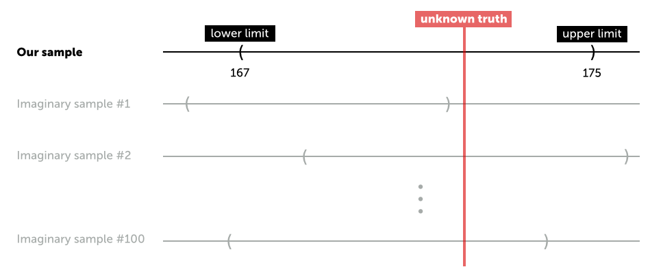
The confidence interval is the most commonly used frequentist tool. It works like this: Let’s say we want to test the hypothesis that the average American male is \( 177 \) cm tall. Let’s also assume that we have a random sample of American males, and the average height of the sample is \( 171 \) cm with a standard error of \( 2 \) cm. The lower limit of a \( 95 \% \) confidence interval is then \( 171-2\ \times 1.96 = 167 \), and the upper limit is \( 171 + 2 \times 1.96 = 175 \).
Since \( 177 \) cm is not inside the confidence interval, we reject the hypothesis that the true average height of all American males is \( 177 \) cm. On the surface, this sounds straightforward, but what does a confidence interval really say? It says that if we were to draw, say, \( 100 \) more samples from the same population, and calculate \( 100 \) different confidence intervals, approximately \( 95 \) of them would contain the true average height of American males.

However, a common interpretation of the confidence interval is: “there is a \( 95 \% \) probability that the true average height is between \( 167 \) cm and \( 175 \) cm.” Here’s why that’s a misinterpretation:
-
In the frequentist paradigm, the parameter (average height) is fixed and unknown, while the data is random. As shown above, the confidence limits vary while the parameter we are trying to make an inference about is fixed and unknown.
-
Thus the true mean is either inside or outside the confidence interval we are observing from our sample - there is no measure of probability here.
-
But before you draw your sample you can say there’s a \( 95 \% \) chance that the resulting confidence interval will contain the true parameter. This is often gets confused with what happens after the sample has been drawn - thus the misperception of the confidence interval
The Credible Interval: The data is fixed, the parameter is random
In the Bayesian paradigm, it’s the parameter that is random while the data is fixed. This paradigm seems logical: it’s not just that the data is fixed in Bayesian inference - the data is fixed in reality, regardless of the paradigm. The one thing we know is that we measured three people’s heights, and they were \( 154 \), \( 187 \), and \( 172 \) cm. There’s no randomness here.
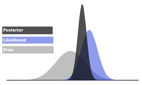
Bayesian analysis is formalized by creating a prior belief and combining it with the likelihood (observed data) to get to the posterior distribution (the final distribution). Priors encode the information that you already have - i.e., they are a way of expressing the results of previous experiments. In other words, yesterday’s posterior is today’s prior.
This is done via Bayes Theorem, which says that the posterior distribution is proportional to the product of the likelihood and the priors:
\[p(\mu \mid x) \propto \mathrm{likelihood} \times \mathrm{prior} = p(x \mid \mu) \times p(\mu)\]
From the posterior distribution we can get the average and the credible interval (i.e. the uncertainty). On the surface, a credible interval looks just like the type of confidence interval we calculated above with an upper and lower limit. But here you can make probability statements such as \( P( \mathrm{true\, height\, in\, interval}) = 95 \% \), which is often what we are seeking. We want to know the probability that the parameter lives in the interval and not the proportion of times we’d expect the true parameter to fall within the interval bands if we ran the experiment a large number of times. This is a more intuitive way to think about uncertainty.
Bayesian Regression is a Shrinkage Estimator
In this section we turn our attention to regression analysis. As stated above, the Bayesian paradigm provides several benefits when fitting regression models.
In a Bayesian regression model the slope coefficients follow prior random distributions:

where the diagonal matrix, \( A \), is called the precision matrix (“tightness” of our priors). Note that this is different from the classical model where the coefficients are unknown constants.
If our priors are normally distributed, the estimator for the posterior mean can be written as:

Note that the posterior is a weighted average of the ordinary least squares estimate (OLS) and the prior belief. Hence, the Bayesian regression model is a shrinkage estimator in the sense that it shrinks the slope posteriors towards the prior means (Bayesian Statistics and Marketing, Rossi et al, 2006).
In fact, Bayesian regression has close ties to regularization techniques. Ridge regression can be thought of as a Bayesian regression where slope priors are normally distributed with means equal to 0. Lasso regression can be interpreted as a Bayesian regression with Laplace priors on the slopes.
Two Commonly Encountered Problems in Regression Analysis
Most of us have heard of multicollinearity (correlated regressors/drivers) and overfitting (e.g., having too many parameters compared to observations). Multicollinearity can cause inflated coefficient standard errors, nonsensical coefficients, and a singular sample covariance matrix. Overfitting leads to models that describe random error noise instead of real relationships. Simply put, both issues can lead to models that do not make sense.
So how do we deal with this in a classical (non-regularized) frequentist model? We can try techniques such as principal component analysis, change time lags (for times series) or even remove business drivers that have non-intuitive coefficients. But such strategies offer little chance of getting an interpretable and robust model if the input data is thin and/or plagued by collinearity. We need to use a more forceful tool - we need to take control of the assumptions of our model.
Bayesian Regression and Regularization: Closely Related Cousins
Like regularization techniques, Bayesian regression offers a potent (but not surefire) weapon against overfitting and multicollinearity. By influencing our model with outside information, we can ensure that the model stays within reason.
For example, let’s say that I am building a regression model to analyze the impact of pricing changes across time. But history is limited, price is correlated with other drivers, and the resulting model is counterintuitive. We don’t have another year to wait for the data to mature, but we do have an outside study which suggests that the average industry price elasticity is \( -0.8 \). In a classical frequentist model, we would have no way of combining these two pieces of information to ensure a useful model, but in a Bayesian model we do.
Now let’s consider the use case where we don’t have a prior, but just want to make sure the model does not go crazy by reducing the prior variance (shrinking). Tightening the variance increases the diagonal of the \( A \) matrix, which in turn increases the diagonal of the \( X^{\prime} X \) matrix during estimation (see formula for the posterior above). This makes our model less susceptible to being plagued by variance inflation and singularity of the sample covariance matrix. This is the same idea employed by the regularization techniques described earlier.
A third use case is the Hierarchical Bayes model where we leverage the hierarchical structure of a dataset (if present) to create a prior structure, and the amount of shrinkage induced is informed by the data. This technique is particularly powerful when estimating effects at a granular level, e.g., at the individual level, because the model allows the slope estimate for an individual to “borrow” information from similar individuals.
Last Word
Bayesian statistics offers a framework to handle uncertainty that is, based on a more intuitive mental model than the frequentist paradigm. Moreover, Bayesian regression shares many features with its powerful regularization cousins while also providing a principled approach to explicitly express prior beliefs.
One criticism of Bayesian methods is that priors can be subjective assumptions. This is true, but it is hard to avoid assumptions in statistical analysis. For example, frequentist methods are typically based on several assumptions such as normally distributed errors, independent observations and asymptotic convergence across infinite repetitions. These can be hard to verify, and violations can impact results in a non-trivial manner. The good news is that the Bayesian paradigm is transparent due to its simplicity. We have Bayes theorem, some priors, and that’s it. You may make the wrong assumption, but it is stated loud and clear and you can work from there as you learn more.
Does this mean that we should all be Bayesians? I would argue that, rather than defining ourselves as frequentists and Bayesians, pragmatism should always be the guiding principle in data science and statistics. Proclaiming to be a pure frequentist or Bayesian is sort of like voting along party lines – i.e., making principle-based decisions that are not always best for the constituents (business partners and customers).
Moreover, Bayesian analysis does have some disadvantages that we need to be aware of:
-
You need a prior, and sometimes you just don’t have one. The wrong prior can send you down the wrong path. We should note that a Bayesian regression with no prior yields the same answer as a classical OLS model.
-
The typical Bayesian problem yields a Markov Chain Monte Carlo (MCMC) problem that’s more complex and expensive than the typical closed-form frequentist solution. However, MCMC is not as hard to deal with as it used to be. These days there are great off-the-shelf packages that can handle just about any MCMC problem.
-
This is not a disadvantage, but an important point: when dealing with large and clean samples, confidence intervals and credible intervals tend to converge.
Being pragmatic means using the right tool for the problem at hand - regardless of what the paradigm is called. At Stitch Fix, for example, we use both approaches every single day. When we’re analyzing a clinically designed A/B test, we use confidence intervals and p-values to make our decision. But we may use Bayesian techniques when we are analyzing less randomized data, such as price and marketing levers.
