The Golden State Warriors won the NBA finals last year and posted the best record in the regular season. Yet some people have argued that their success was based on luck and that playing “small ball” is a recipe that only works in the regular season.
Here at the Stitch Fix algorithms team we have several devoted Warriors fans and hence we had to investigate these claims – from a data science point of view, of course. Our analyses revealed two key findings, which we will discuss in this post:
- The success of the Golden State Warriors last year was indeed not based on luck, but rather a diverse and efficient roster coupled with smart coaching.
- If Kevin Love and Kyrie Irving had been healthy during the finals, Golden State would still have won – although it would likely have been a very close seven-game series.
Methodology – High Level View
The basic mental model behind this post is the following: if we can generate matchup-level predictions that are blind to recent win/loss momentum, and these predictions also rank GSW as the best team last year, then the success was meant to be.
In order to model this, we wanted to understand the impact of player archetypes on a team’s probability to win a given matchup. Specifically, we modeled how the allocation of minutes across archetypes – which depends on the roster and coaching decisions – affects a team’s ability to win basketball games in the NBA.
In other words, this approach focuses on the DNA of the team, rather than momentum and synergistic events on the court. Thus, we’re essentially investigating if Golden State had the best DNA last season.
Step 1: Player Archetypes
Derive player archetypes (clusters) using k-means clustering based on player-level box score data from the 2011–2012 and 2012–2013 seasons. The archetypes are simply centroids based on player-level statistics and can be mapped to any player in future seasons.
Note that the archetypes are essentially a simplified view of player performance. This creates robustness (larger sample sizes than individual players) and we avoid (to some degree) modeling the presence of a single superstar, which would not agree with our basic mental model.
Step 2: Predicting the Outcome of a Matchup
While the k-means clustering in step 1 discovers archetypes in an unsupervised fashion, the model built in this step estimates the importance of the various archetypes in terms of predicting wins and losses:
- For a given matchup in the 2014–2015 season (last season): Determine each player’s archetype based on their statistics over the prior 90 days.
- Based on the differences in minutes allocated to the archetypes, use a regression model to predict the winner of the matchup. This essentially means that the prediction is based on a team’s ability to have a surplus of minutes allocated to powerful archetypes.
Note that this model does not know how well the team is doing at any point in time, or how well the team did subsequently. Moreover, it does not know the interactions between the players as the data used is based on box scores. In other words, the model is blind to synergy and momentum.
On the other hand, the model does know how many minutes the coaches allocate to each archetype, which means that we’re effectively controlling for injuries. Also, the difference in minutes allocated does partially reflect the quality of the coach.
Step 3: Compare to Reality
Compare the predictions for each matchup to the actual outcomes. This step is the crux of the analysis. As stated above, our argument is based on the premise that, if this simple model agrees with reality, then the success was not due to luck or some magic synergy-based momentum.
Player Archetypes
As mentioned above, the archetypes were created using k-means clustering of box scores from the 2011-2013 seasons. The following variables were used to form the clusters:
- assists
- defensive and offensive rebounds
- turnovers
- steals
- points
- minutes
- three-pointers made
- field goals made
- field goal percentage
- free throws made
- free throw percentage
- blocks
- share of minutes played
- efficiency (EFF as defined by the NBA)
We aimed to capture \(80–90\%\) of the total sum of squares and ultimately settled on 50 archetypes for players that play more than 8 minutes per game (the average excludes games where they did not play at all), and one cluster for the players that play less than 8 minutes (51 clusters in all). Note that, in a given season, there are around \(400–450\) players that play more than 8 minutes per game.
Note that the archetypes are simplifications of the actual players — they’re simply a set of centroids from the k-means clustering. In order to understand the clusters better, we created a heatmap and mapped the 25 most active archetypes (in terms of minutes played) to players during the 2014-2015 season. The player names on the right side show the most representative players from each cluster during the 2014-2015 season. The values in the heatmap are for the centroids of each cluster.
The heat map shows that Stephen Curry — the season MVP — belongs to an efficient archetype with a high average of three-pointers made. It also shows that the closest archetypes are represented by players such as Chris Paul and Kyrie Irving.
Predicting the Outcome of a Matchup
This is where we translate minutes allocated across player archetypes into the probability of a given team winning a matchup by estimating the importance of the various archetypes. We’ll discuss this model by covering three overall sections:
- The predictive variables (i.e., derived features) used in the model.
- Model estimation details.
- Validation approach and results.
Predictive Variables
The regression model used in step 2 above is based on the simple idea that the winner of a matchup can be predicted by comparing minutes allocated to the different clusters during the game. Specifically, for each team we create the following variables:
Derived variables for team 1:
\(X_1 = \text{ % of minutes allocated to cluster 1}\)
\[X_2 = \text{ % of minutes allocated to cluster 2}\] \[\vdots\] \[X_{51} = \text{ % of minutes allocated to cluster 51}\]Derived variables for team 2:
\(Z_1 = \text{ % of minutes allocated to cluster 1}\)
\[Z_2 = \text{ % of minutes allocated to cluster 2}\] \[\vdots\] \[Z_{51} = \text{ % of minutes allocated to cluster 51}\]From these variables we capture the differences between the two teams, during the given matchup, by constructing the “delta variables” given by
\[D_{1} = X_{1} – Z_{1}, D_{2} = X_{2} – Z_{2}, \ldots, D_{51} = X_{51} – Z_{51}. \nonumber\]Estimation
The model is a logistic regression model given by
\[\log(P(\text{team 1 wins})\,/\,P(\text{team 2 wins})) = \alpha + \sum_{j=1}^{51} \beta_j D_j + \beta_{52} H, \nonumber\]where \(H\) is a pooled home court indicator that is not specific to a team (using team-specific home court advantage would break the mental model of the analysis). The coefficients, \(\beta\_1, \ldots, \beta_{51}\), are updated on a 90-day rolling basis using L1 regularization (lasso) to promote sparseness and reduce the chance of overfitting (due to the large number of parameters compared to data points). Thus, we are solving the problem,
\[\min_{\alpha, \beta} \left( \frac{1}{N} \sum_{i=1}^{N} L( y_{i}, \alpha, \beta_{1}, \ldots, \beta_{52}) + \lambda \sum_{j=1}^{52} | \beta_{j} | \right),\]where \(L(\cdot)\) is the negative log-likelihood function for a standard logistic regression and \(\lambda\) determines the level of penalty applied to the model. This can be done using the glmnet package in R, which also allows for estimation of \(\lambda\) using v-fold cross-validation.
Coefficient Updates
As mentioned, we are re-estimating every day during the season using a trailing 90 game-day window (i.e., excluding days with no games). The justification behind this is the following:
-
A given archetype may affect the games differently throughout the season. We want the model to be adaptive. In the beginning of the season, predictions rely on the previous season. As the season progresses, the predictions rely solely on historical games from the current season.
-
By dynamically updating models and using a fairly large number of archetypes, it is likely that we are picking up some latent momentum trends, which are not part of our basic mental model. However, that is pretty much unquantifiable and we have decided to live with that risk.
Validation
The probability of team 1 winning the matchup is given by
\[p = \left(1 + \exp(-\hat{\alpha} - \sum_{j=1}^{51} \hat{\beta_j} D_j - \hat{\beta}_{52} H)\ \right)^{-1}, \nonumber\]and we predict that team 1 will win when \(p>0.5\). Note that for a given 90-day window, several variables can have coefficients that have been shrunk to \(0\) – i.e., deselected by the L1 regularization.
The model was validated using one-day-ahead validations, which means that we are using historical data from the previous 90 game days to predict the outcomes of the next day.
Using this validation scheme, the accuracy in terms of correctly guessing the outcome of an individual game (across all teams) was \(63\%\) for the first half of the season and 66% for the second half (including playoffs). The area under the ROC curve for the first half is \(0.68\) and \(0.71\) for the second half. Overall, these are decent validation numbers given the simplicity of the model, and it is good to see that the model got better over time.
For Golden State, the accuracy during the regular season was \(81\%\) and during the playoffs was \(76\%\). In fact, the model tends to do better for more “extreme” teams. For example, the model correctly predicted \(75\%\) of the Laker’s games – a team with poor DNA last year. For San Antonio, the accuracy was closer to \(60\%\).
In terms of ranking teams by winning percentages – i.e., getting the overall number of wins right for the last season, but not necessarily each individual game – the model does quite well. We’ll see this in the next section.
Comparing to Reality
This is where we test our hypothesis. As stated above our mental model is that, if the “simpleton” model agrees with the outcome of last season as well as the playoffs, Golden State’s success was meant to be.
It turns out that the model back-predicted that Golden State would indeed have been the best team in the season (using one-day-ahead predictions). In fact, the model predicted a 78-win season! Moreover, the model predicted that Golden State would have won all four playoff series handedly. Hence, we conclude that the success of the Golden State Warriors was not luck – they had the best DNA.
The table below shows the predicted and actual winning percentages for the 2014-2015 season. It also shows the predicted ranks (“Rank”) and the difference between the predicted and actual ranks (“Rank Diff”). A negative rank difference means that the model thinks the team should have been better than it really was (e.g., Portland). A positive rank difference means that the team overperformed relative to the model’s expectations (e.g., San Antonio).
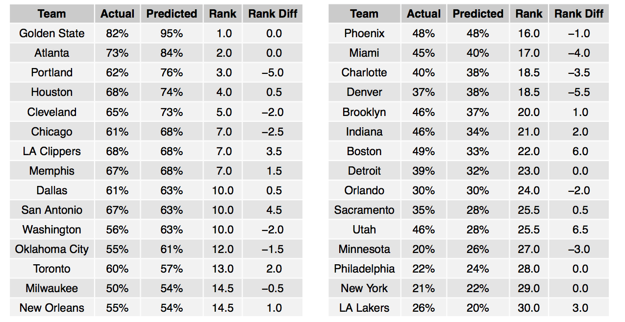
Next, we looked at how well the model did during the playoffs. As we can see, the model was slightly optimistic for the Memphis and Cleveland series. For Memphis, the model would have predicted a sweep and for the Cleveland series the model only projected one loss.

So, Why is Golden State a Good Team?
The regression model and archetype analysis confirmed two things Warriors fans already know: Steph Curry is in a league of his own, and the team has the right players available at the right time.
Steph Curry is in a league of his own
According to the model coefficients, Curry belongs to an important archetype. Additionally, Curry was the only player who consistently matched this archetype in every game throughout the 2014-2015 season. In other words, Curry is consistent, efficient and helps his team win. For comparison, Damian Lillard only matched the same archetype as Curry for 30% of the 2014-2015 season.
The right players at the right time
Golden State were able to allocate more minutes than its opponents to several key archetypes. This suggests that Golden State’s roster is deep and varied – i.e., the team has strong DNA – and that the coaching staff knows how to distribute minutes efficiently and to adapt to opponents.
The charts below help illustrate this for the 2014-2015 season: the “width” of the bars illustrates the importance of the archetypes and the length illustrates the amount of surplus in minutes allocated (these are the \(D_j\) variables in the logistic regression model). Note that the Timberwolves allocated more minutes than its opponents to lower performing archetypes, which explains why they only won \(20\%\) of games last year.
What if Kevin Love and Kyrie Irving Had Played?
We’ve all heard the speculations that Cleveland would have won if Kevin Love and Kyrie Irving had been healthy. Naturally, we thought this would be a good question to model. Here is how we went about it:
- Identified the only game last season where all key players from both Golden State and the Cavaliers were healthy. This was on February 26, 2015 and the game was played in Cleveland. Cleveland won, although the model predicted a Golden State win. This game gave us an idea of how the minutes are allocated when all players are healthy.
- Moved the game to the playoffs and ran it through the model. Recall that the model is updated on a 90-day basis and players are remapped to the archetypes. Thus, the prediction from February 2015 will not be the same as the prediction in June 2015.
This analysis painted an interesting, yet credible story: the model back-predicted a \(54\%\) chance that the Cavaliers would have won in Cleveland and \(53\%\) chance that Golden State would have defended its home court. Based on these predictions, Golden state would be favored to win the series by a very narrow margin. In other words, if Kevin Love and Kyrie Irving had been healthy, it would likely have been a very close, hard-fought seven-game series with Golden State ultimately prevailing due to home court advantage. Could it have gone both ways? Of course, but we had to pick a winner.
Other Potential Applications
If we were to use this model going forward — not for back-predicting to prove a hypothesis — we’d have to make assumptions about minutes played for each player and then map those minutes to archetypes. This would create an interesting what-if scenario environment where coaches can play with minute allocation scenarios prior to a game, just like businesses run scenarios during quarterly and annual planning.
Last Words
It goes without saying that no bullet proof argument exists for whether or not Golden State’s success was due to superior DNA or luck. Our approach is just one view and it’s possible that another group of data scientists would arrive at a different answer. No one will ever know.
However, based on this analysis, as well as an amazing 5-0 start to the current season — including a win over the Clippers whose coach has been advancing the “luck argument” — we feel good about Golden State’s chances of repeating the success of last season. In fact, only four other teams in NBA history have started 5-0 and the cumulative point differential so far this season is the fifth-best margin through five consecutive games in NBA history.
The DNA (archetype composition) is pretty much the same as last season, but the Warriors may be even better this season. We plan to keep monitoring this by creating ongoing predictions and insights using this model. Stay tuned.