Introducing our Hybrid lda2vec Algorithm

The goal of lda2vec is to make volumes of text useful to humans (not machines!) while still keeping the model simple to modify. It learns the powerful word representations in word2vec while jointly constructing human-interpretable LDA document representations.

We fed our hybrid lda2vec algorithm (docs, code and paper ) every Hacker News comment through 2015. The results reveal what topics and trends are changing as the community evolves while still maintaining word2vec’s most remarkable properties, for example understanding that Javascript - frontend + server = node.js. Code and documentation to reproduce this post is available here.

Hacker News Trends

Imagine we ran Hacker News like a profit-seeking company. We’d have questions like: How does the focus of the community shift over time? What topics get on the front page with the most points? Let’s use lda2vec to analyze the HN corpus.

Trends

One of results you’ll get out of lda2vec is a visualization of topics and the most frequent words in those topics:

Using this tool we discover that topic 5 pops up with words like (bing, g+, cuil, duck duck go) – so we’ll call this the search engine topic. And then topic 38 has phrases like (snowden, terrorist, assange FISC, ACLU), so we’ll call this the national security topic. After doing this for the remaining 38 topics you might get a list that looks like this. So assigning a name to a topic requires a human touch and an hour of your time, but the pyLDAvis tool is tremendously helpful. Once labelled, we start analyzing the topics. If you’re curious how the sausage is made and would like to improve on it, the full analysis notebook is here.

Rising rents

Housing prices around the US have risen steeply in the last few years and especially in the Bay Area. Perhaps as a response, HN topics reflecting on housing are on the rise:

HN Job Postings

Job postings for remote engineers have plateaued, but general job postings seem to be slowly climbing.

Civil Rights

The topic of civil rights has ebbed and flowed over time, but it suddenly spiked with Edward Snowden’s arrival on the scene in the middle of 2013. Since then, topics in internet security and authentication have stabilized at higher levels.

So this kind of analysis can yield interpretable topics that help humans understand what’s being written without much reading on our part. Maybe the folks behind Hacker News want to evolve the site by encouraging more job hiring posts, or maybe they’d like to devote special site features to housing or more security features. That’s the kind of analysis we need to effectively steer our companies: more insight, less black box. And this is the most practical difference in use cases between word2vec and LDA – the latter has ability to summarize text data in a way that better helps us understand phenomena and act at a high-level.

Algebra on words

Not only do we get topics over text just as in LDA, but we also retain the ability to do the kind of algebra on words that word2vec popularized, but specialized to the HN corpus:

Jeff Bezos and Mark Zuckerberg are the CEOs of Amazon and Facebook respectively:

Hacker News and StackOverflow are highly trafficked websites with technical content in the form of articles and questions respectively:

VIM is a powerful terminal-bound editor and Photoshop is well known for its graphical editing abilities:

The Surface Pro and Kindle are tablet-like devices released by Microsoft and Amazon respectively:

And slightly more whimsically:

If you’d like to play around with these at home and ask your own questions it’s easy! Checkout the short intructions and a guide that will help you download the vectors and get you started here.

Mixing LDA + word2vec = lda2vec

lda2vec combines the power of word2vec with the interpretability of LDA. That recipe for calls for three architectural changes:

1. Combining global document themes with local word patterns
2. Dense word vectors but sparse document vectors
3. Mixture models for interpretability

Global & local

At its heart, word2vec predicts locally: given a word it guesses neighboring words. At Stitch Fix, this text is typically a client comment about an item in a fix:

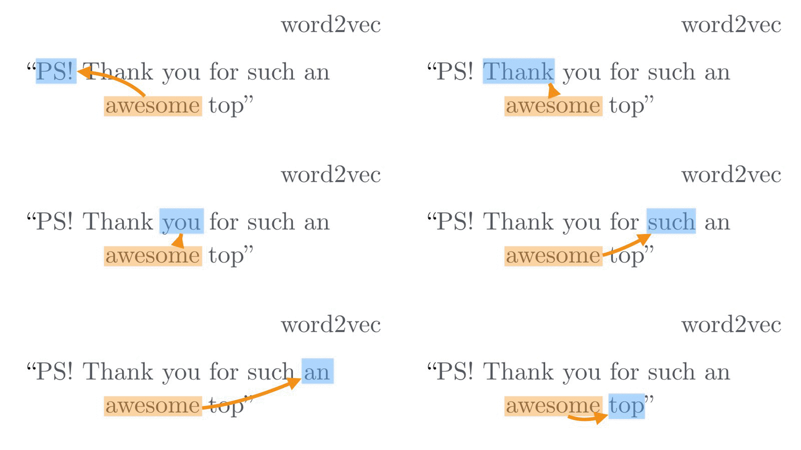
In this example, word2vec predicts the other words in a sentence given the central pivot word ‘awesome’ and repeats this process for every pair of words in a moving window. Ultimately this yields wonderful word vectors that have surprisingly powerful representations. LDA on the other hand predicts globally: it learns a document vector that predicts words inside of that document. And so in one of our client’s comments about their fix:

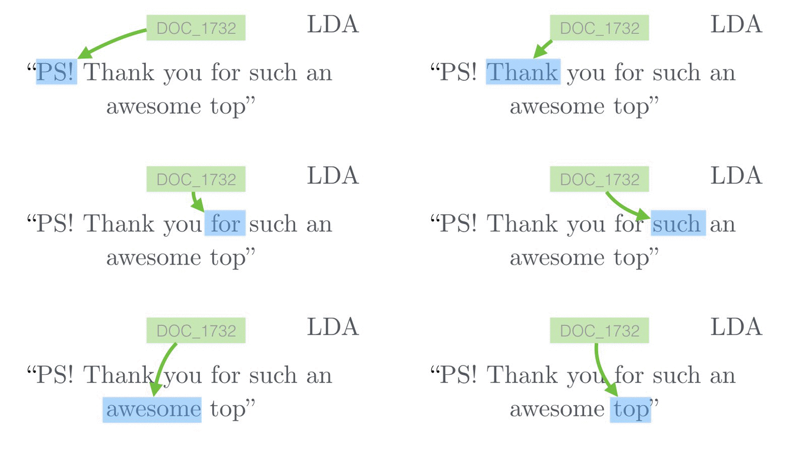it predicts all of the words using a single document-wide vector and doesn’t capture more local word-to-word correlations.

lda2vec predicts globally and locally at the same time

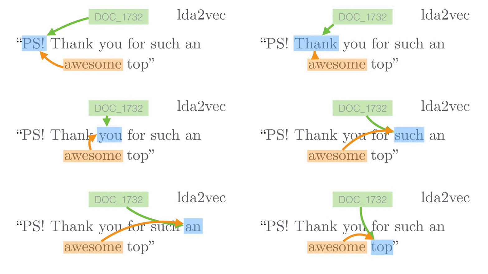
by predicting the given word using both nearby words and global document themes.

The hope is that more data and more features helps us better predict neighboring words. Having a local word feature helps predict words inside of a sentence. Having a document vector captures long-range themes beyond the scale of a few words and instead arcing over thousands of words.

Representations

Dense distributed vectors

Word vectors, despite having the amazing ability to sum concepts together (e.g. silicon valley ~ california + technology and uber ~ taxis + company) are several hundred dimensional vectors that are extremely difficult to interpret for humans. A typical word vector looks like a dense list of numbers:

And this vector, alone, is meaningless. It indicates an address more than a quantity. So the first element in this vector isn’t -0.75 of something. It helps to think of it as being at the coordinate -0.75 with the property that any other vector close to that -0.75 will be similar.

Sparse simplex vectors

We can decipher what the word vector addresses mean by looking at their neighborhoods, but LDA document vectors are quite a bit easier to interpret. A typical one looks like this:

This vector tells us that this document is 0% in most topics, and then perhaps 9% in the bitcoin topic, 78% in programming, and 11% in the national security.

But there’s a few things to note: the vector is sparse – most of the elements are close to zero. The intuition is that this vector has a few critical properties and the rest are close to irrelevant. The LDA vector is much easier to reason about too: the document could have been in a hundred different topics, but we designed the algorithm to encourage mixtures made up of just a few properties. This concentration in a few topics makes it easier to read and easier to communicate.

Another critical difference is that the elements sum to 100% and are all non-negative (e.g. the vector lives on the ‘simplex’ ). And this constraint is great: otherwise it would have been hard to grok that a document is -0.75 * bitcoin + 2.2 * programming – what does a negative 0.75 bitcoin document even mean? Much easier to understand is that the document is 0% bitcoin and 78% programming. Both kinds of vector representations are mathematically plausible, and to a machine this makes little difference. But as a scientist, if you can, choose models made for humans!

Mixtures

Another ingredient in LDA is that it is a mixture model; each document will have mixed membership in a core set of topics. Whereas a 300D word vector can be similar or dissimilar to other words in three hundred different ways, a document has to carefully choose only a few topics to belong to. This is where lda2vec exploits the additive properties of word2vec: if Vim is equal to text editor plus terminal and Lufthansa is Germany plus airlines then maybe a document vector could also be composed of a small core set of ideas added together. lda2vec still must learn what those central topic vectors should be, but once found all documents should just be a mix of those central ideas.

In our Hacker News example, lda2vec finds that a document vector describing Google Reader shutting down has a topic mix of 27% bing, google, and search engines + 15% karma, votes, comments, stories, rss + 8% of online payments, banking, domain registration, user accounts and smaller bits of other topics.

Technical Details

For a quick summary of how the algorithm works, check out the animation below which walks you through the major design decisions behind lda2vec:

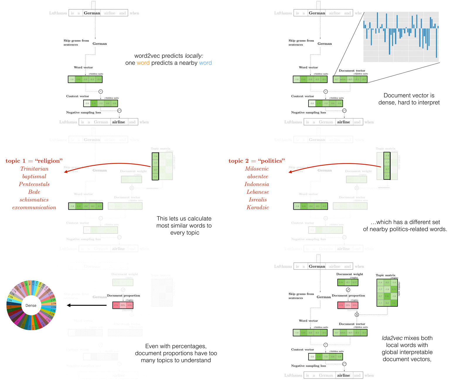
Objective Function

Similar to word2vec’s skipgram negative-sampling (SGNS) algorithm, we’ll start by trying to discriminate pairs of (context j, word i) that appear in the corpus from those randomly sampled from a ‘negative’ pool of words and contexts. That objective function is:

\begin{equation} L = \sigma(\vec{c_j} \cdot \vec{w_i}) + \sigma(-\vec{c_j} \cdot \vec{w_{negative}}) \end{equation}

This loss function is minimized when you distinguish (\(\vec{c_j}, \vec{w_i}\)) pairs from the observed data and separate them correctly from ‘negatively’ sampled pairs drawn at random. Unlike trying to predict the next word (as in softmax regression) this has the attractive property of controlling for the base rates of each token’s popularity. This helps us learn word vectors while removing the effect of overall prevalence and focusing on learning just the vector conditional on a context.

The twist in lda2vec is that we’re going to extend what “context” means. In word2vec, the context vector is simply the central pivot word vector (\(\vec{c_j} = \vec{w_j}\)). In LDA, context isn’t a word at all and is replaced with a document vector (\(\vec{c_j} = \vec{d_j}\)). In lda2vec, the context is the sum of a document vector and a word vector:

\begin{equation} \vec{c_j} = \vec{w_j} + \vec{d_j} \end{equation}

The context vector will be composed of a local word and global document vector. The intuition is that word vectors can be meaningfully summed – for example, Lufthansa = German + airline. If as we’re scanning a document the jth word is German, then we might expect to see similar words: French, Spanish, and English. But if the document is specifically about search engines, then the document vector might shift those probabilities slightly closer to the combination of German with airline and this get us predictions that are a bit more fine-tuned to match a document’s theme. When added together German + airline the scores for words similar to both - like Lufthansa, Condor Flugdienst, and Aero Lloyd - all jump up.

If we stopped here, we’d have something similar to paragraph vectors (see also gensim’s implementation here). But despite impressive benchmarks these document vectors are still difficult for me to interpret, so let’s project them on to a mixture:

\begin{equation} \vec{d_j} = a_{j0} \cdot \vec{t_0} + a_{j1} \cdot \vec{t_1} + … \end{equation}

This decomposes a document vector into a set of bases \(t_0, t_1, ...\) that will form our topic vectors. Each weight \(a_{jk}\) will be a scalar that tells us how much of each topic we need to add in to reconstruct the document vector. In practice, we use a softmax transform to map numbers from the real vectors onto the simplex, which forces our weights to sum to 100%. Formulating the mixture in this way also ensures that topic vectors and word vectors live in the same space and so we keep the ability to calculate what words are most similar to \(t_0\). If we compute \(t_0\)’s neighbors using \(similarity = t_0 \cdot w_j\) we might find that the most similar words are NSA, FBI, FISA, and WikiLeaks. And so I might call \(t_0\) the national security topic.

The weights change for every document, but the topics are shared among all documents. For example for three documents this decomposition looks like:

\begin{equation} \scriptsize \vec{d_0} = 0\% \cdot national\ security + 0\% \cdot operating\ systems + 10\% \cdot programming + … \end{equation}

\begin{equation} \scriptsize \vec{d_1} = 88\% \cdot national\ security + 0\% \cdot operating\ systems + 0\% \cdot programming + … \end{equation}

\begin{equation} \scriptsize \vec{d_2} = 15\% \cdot national\ security + 2\% \cdot operating\ systems + 0\% \cdot programming + … \end{equation}

Once we go through the exercise of labeling each topic, the mixture vectors then become fairly interpretable.

The final ingredient is to encourage the weights to look like a sparse Dirichlet distribution. Sampling from the Dirichlet can get involved, but conveniently measuring and optimizing the likelihood is extremely simple:

\begin{equation} \Sigma_k (\alpha_k - 1) log p_k \end{equation}

(Note that we’ve thrown out the terms independent of document weights. Furthermore, \(\alpha_k\) is usually a constant set to \(\frac{1}{number\ of\ documents}\), and so the only variable to optimize is the document-to-topic proportion, \(p_k\).)

This simple likelihood makes projections onto our latent topic basis sparse. Without this sparsity-inducing term the document weights tend to have evenly spread out mass which makes reading the document vectors as difficult as word vectors. Furthermore, the topic vectors that the document weights couple to are also junk when not imposing a Dirichlet likelihood. Curiously, without this term the topic vectors are poorly defined and seem to produce incoherent groups of words.

At the end of the day, the final objective function looks like this:

\begin{equation} \mathcal{L} = \Sigma_{word\ pairs\ (i, j)} [\sigma(\vec{c_j} \cdot \vec{w_i}) + \sigma(-\vec{c_j}\cdot \vec{w_{negative}})] + \Sigma_{documents\ k}\ log\ q(d_k|\alpha) \end{equation} \begin{equation} \vec{c_j} = \vec{w_j} + \vec{d_j} \end{equation} \begin{equation} \vec{d_j} = a_{j0} \cdot \vec{t_0} + a_{j1} \cdot \vec{t_1} + … \end{equation} \begin{equation} q(d_k|\alpha) = \Sigma_k (\alpha_k - 1) log a_k \end{equation}

The first line discrimates observed word-context pairs from negatively-sampled ones and adds in a regularization for document weights. The second line indicates that a context is the sum of a word vector and the document vector. The next line projects latent document weights onto topic vectors, and the final line defines the Dirichlet likelihood for those weights.

Experiment: regularize the covariance

The advent of automatic differentiation frameworks like Chainer make it extremely simple to alter and refine models. This let’s us try to fix problems we see in our own or others’ models.

Sampling from a Dirichlet enforces a strict covariance scheme (which means topics try to be roughly orthogonal). lda2vec on the other hand optimizes a Dirichlet likelihood instead of sampling from it, and can suffer from highly correlated topics that are nearly identical. For example, there are three job posting topics that to my eye are very redundant. One idea on how to fix this is to regularize the covariance. And one way to do that is to penalize the determinant of the topic covariance matrix; the covariance matrix let’s you know how much topic vector i correlates with topic vector j and the determinant effectively penalizes complexity in that matrix. It’s simple to add to the loss function a matrix regularzation term:

\begin{equation} \mathcal{L} += log(det\mid\Sigma_{ij}\mid) \end{equation}

where

\begin{equation} \Sigma_{ij} = (t_i - \mu_i) ( t_j - \mu_j). \end{equation}

I’m still evaluating whether this is a good idea or not, but the point here is that you can easily modify the model – the crux of it is just 90 lines of code. Previously, these kinds of models took substantial effort to find approximations and derive iterative updates – but now you have the option to tinker and tweak prototypes without deriving a new method every time.

This ability to modify models and to quickly swap out architectures and try out new ideas cheaply is what makes automatic differentiation tools like Chainer (and of course, AutoGrad, Theano, Stan, Torch, Neon, etc.) amazingly useful.

Should I use lda2vec?

Probably not! At a practical level, if you want human-readable topics just use LDA (checkout libraries in scikit-learn and gensim). If you want machine-useable word-level features, use word2vec. But if you want to rework your own topic models that, say, jointly correlate an article’s topics with votes or predict topics over users then you might be interested in lda2vec.

There are also a number of reasons not to use lda2vec: while the code has decent unit testing and reasonable documentation, it’s built to drive experimentation. It requires a huge amount of computation, and so I wouldn’t really try it without GPUs. Furthermore, I haven’t measured lda2vec’s performance against LDA and word2vec baselines – it might be worse or it might be better, and your mileage may vary.

Bottom Line

Deep learning approaches have spectacular performance on supervised tasks, but their data products are usually not designed with humans in mind. I think that makes it difficult to understand your system, to move science forward, and to communicate your results. What lda2vec demonstrates is that you can at least try to build models with interpretable results very simply – building a sparse mixture isn’t very much work in today’s frameworks. Build models for humans!

More info

Similar models exist:

1. Neural Variational Document Model (code, paper). This model uses the varitional autoencoder infrastructure to construct bag of words representations over documents. With respect to lda2vec, it builds performant (but dense) document vectors and throws out word-to-word relationships.
2. I just learned about these papers which are quite similar: Gaussian LDA for Topic Word Embeddings and Nonparametric Spherical Topic Modeling with Word Embeddings. Both models strive to incorporate LDA and word2vec and get state of the art results, but bolt-on pretrained word embeddings instead of learning them jointly. Still, both papers introduce new and clever ideas that could yield improved topic models.