Here at Stitch Fix we work on a wide and varied set of data science problems. One area that we are heavily involved with is operations. Operations covers a broad range of problems and can involve things like optimizing shipping, allocating items to warehouses, coordinating processes to ensure that our products arrive on time, or optimizing the internal workings of a warehouse.
 One of the canonical questions in operations is the traveling salesman problem (TSP). In its simplest form, we have a busy salesperson who must visit a set number of locations once. Time is money, so the salesperson wants to choose a route that minimizes the total distance traveled. It is not so hard to imagine these path optimization problems occurring within warehouses where people (‘pickers’) need to navigate aisles and fill orders as they go.
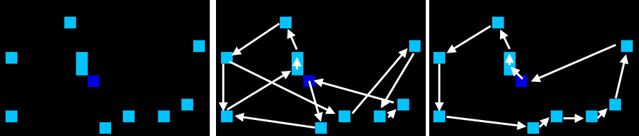
As an example of a TSP, we can see below on the left we have the salesperson (dark blue) and all the places they must visit (light blue). The center panel shows an example of a bad tour: there is backtracking and the route taken is not optimal. We can compare that to an optimal tour on the right, which is much more efficient.
The simplest way to find an optimal route is to try all combinations of locations and then choose the one that gives the smallest distance. However, it is easy to see that the number of combinations grows exponentially, and for 60 cities there are already more possible combinations than atoms in the universe. Having efficient algorithms that can find solutions becomes very important for solving the TSP. The TSP occurs widely in science, nature and industry, and is in fact part of the P=NP millennium problems set out by the Clay Institute for Mathematics.
How do we solve the TSP? There is a plethora of ways to solve the TSP. These include algorithms which give exact and approximate tours as well as deterministic and stochastic algorithms. They all involve minimizing the following cost function
\[\min \sum_{i,j} d_{ij} X_{ij},\]where \(d_{ij}\) is the distance traveled between two locations \(i\) and \(j\) and \(X_{ij}\) is a binary variable indicating if the tour includes traveling between \(i\) and \(j\). This alone is not enough to solve the TSP, and we need to include two additional constraints, one that says the salesperson should enter and exit a location only once, and one that says the tour must be fully connected (no sub-tours).
I am not going to talk about the more traditional methods of solving the TSP, but instead demonstrate a slightly more convoluted (but interesting) way, that easily extends to complicated real-world problems.. For references to the more traditional ways to solve the TSP see here and here, while a couple of alternate ways can be found here and here.
TSP as a game
One way to think of the TSP problem is to draw an analogy with the famous game Pac-Man. In Pac-Man the aim is to collect as many points as possible while navigating a maze and avoiding ghosts - it is not dissimilar to the TSP (minus the ghosts). With this inspiration we can look to solve the TSP in another way - by treating it as game (this is similar to the Physical Travelling Salesman Problem). In 2015 a famous demonstration showed that an algorithm was able to achieve human level performance in a number of Atari games (including Pac-Man). This was made possible by deep \(Q\) learning - a variant of Reinforcement Learning (RL). In \(Q\) learning, the aim is to learn a \(Q\) function which gives the expected future reward (think score) given the current state (pixels from Pac-Man) if a particular action (up, down, etc.) is taken. The action that has the highest expected future reward is selected. So if RL can learn to play Pac-Man, can we use it to solve the TSP?
Let’s start with a very simple warehouse, one that is pretty empty and only has a few items. We want the picker to collect all of the items, giving a reward for every item collected and subtracting a small penalty for every move taken - the highest score will come from the route that collects the items in the shortest number of moves (exactly what we want for the TSP).
Below is a very simple example demonstrating the results of training the algorithm. We can see it does a pretty reasonable job of collecting the items.
We have control of the environment, so let’s add more items.
Again, it does a pretty good job of collecting all the items in a pretty efficient manner. It has essentially solved the TSP (albeit for a small number of items). It is important to note here that we have not coded any kind of heuristics about how the picker should move when it is near an item, the algorithm has learnt through playing many games.
How does it learn?
So how is it learning? In this variant we are trying to learn our \(Q\) function through many games. It takes in the current state (the pixels) and outputs expected future rewards for each action (up, down, left and right). Initially, the estimate for \(Q\) is very wrong, but gets progressively better as many more games are played. In the case of a small set of states and actions, it is possible to simply search and fill in all possible combinations and map \(Q\) using a table. However, in many cases, the space is much too large to do this. Instead, here the \(Q\) function is approximated by a convolutional neural network with its parameters updated as the games are played.
Deep Q learning
In the case of our picker above, the goal is to select actions that maximize cumulative future reward (not just selecting an action that will maximize immediate reward).
The optimal action-value function is given by
which is the maximum sum of rewards \(r_t\) (discounted by \(\gamma\)) at each time \(t\) achievable by a ‘policy’ \(\pi\) (the pickers behavior), after an observation \(s\) (the pixels) and taking an action \(a\).
If we have the optimal \(Q\) function, then it answers the question of ‘given my current state \(s\) what action should I take that will maximize my future reward?’. The \(\gamma\) factor allows a choice between how short sighted we want to be - \(\gamma\) = 0 would simply be choosing actions that maximize immediate reward, while \(\gamma\) close to 1 encourages actions for longer term rewards.
The optimal \(Q\) function can be decomposed as follows
\[Q^*(s,a) = \mathbf{E_{s'}}[r + \gamma \max_{a'}Q^*(s',a')|s,a],\]which is the known as the Bellman equation. This is basically saying that the current expected future reward for state \(s\) is given by the reward \(r\), observed when moving from state \(s\) to \(s'\), plus the maximum estimated expected future reward from the new state \(s'\) (i.e. predicting the future).
So in the ideal world, if we have \(Q^*\) then the agent can act optimally by choosing the policy \(\pi\) via
\[\pi^*(s) = \underset{a}{\operatorname{argmax}} Q^*(s,a),\]which is saying that actions are chosen that will give the greatest future return. In reality, when learning the \(Q\) function, the actions will be somewhat random as we do not yet have a good estimate for \(Q\). The agent will do some exploration of the state space but will quickly follow a ‘greedy’ policy as \(Q\) converges and the amount of exploration will decrease. To ensure adequate exploration of the state space, an additional parameter \(\epsilon\) is introduced, which is the probability of choosing a random action rather than the action given by \(Q\). This value is gradually annealed from 1 to some minimum value (e.g. 0.1) as training progresses and is known as \(\epsilon\)-greedy exploration.
In deep Q-learning, the \(Q\) function is parameterized with a convolutional neural network as \(Q(s,a,\theta)\) with network weights \(\theta\). The Bellman equation is then used to iteratively update the \(Q\) function by minimizing the following loss function
\[L(\theta) = (r+\gamma \max_{a'} Q(s',a',\theta) - Q(s,a,\theta))^2,\]with respect to the network parameters.
In reality, several other things need to be done to make deep-Q learning work reliably for harder problems. The first is that rather than simply updating the network parameters using the most recent states, a history of experiences is stored (\(s,a,r,s'\)) and randomly sampled in batches (‘experience replay’). This helps to de-correlate the update and also allows better use of the data (as it can be used more than once). The second step is to modify the loss function to be
\[L(\theta) = (r+\gamma \max_{a'} Q(s',a',\theta^{-}) - Q(s,a,\theta))^2,\]where the network parameters \(\theta^{-}\) are a copy of the network at some prior iteration. Another important aspect is that rather than simply feeding in a single time step when obtaining \(Q\) values, we can actually design the network to take into account an arbitrary number of previous steps (thus modifying our \(s\) and allowing us to capture concepts like velocity). Since the original implementation there has been a plethora of improvements. Examples are modifications to the loss function
\[L(\theta) = (r+\gamma Q(s', \underset{a'}{\operatorname{argmax}} Q(s',a',\theta),\theta^{-}) - Q(s,a,\theta))^2,\](double deep Q learning), or by ‘prioritized replay’ - where the probability of drawing previous replay tuples (\(s,a,r,s'\)) is weighted by their error
\[\|r+\gamma \max_{a'} Q(s',a',\theta) - Q(s,a,\theta)\|.\]One final interesting thing to consider is how to setup the network to predict the \(Q\) values. If we want to know what \(Q\) is for a particular state and action we could feed these into our our network and obtain a single value, repeating for all actions. However, this is inefficient and does not scale well with the number of actions. Instead, due to the flexibility of neural networks, all the action values can be predicted at once, going from a single output value to one that has \(N\) (corresponding to the number of actions) output values. Although there have been many advancements since the original DeepMind paper, these are the building blocks of how RL can be used to train a neural network to control our picker (example code an be found here1).
Back to the salesman
But this seems like a pretty roundabout way to solve this problem. So why would we use something like RL? We can see that in this case we have exquisite control over the environment. What if we have some obstacles to navigate?
So now our picker has to collect all the items in the shortest time while navigating our new obstacles.
Let’s complicate the scenario by including multiple sales-people who need to avoid collisions. Below we see multiple agents collecting items within the warehouse, all controlled by the same network. So now it starts to be apparent that there may be some usefulness in such an approach as RL. With multiple agents that are moving constantly it becomes much harder to solve and determine the optimal route. Thinking back to the original formulation, how do we calculate \(d_{ij}\) in a dynamic environment?
Let’s make the warehouse really crowded!
Now we have 4 pickers trying to collect their items as efficiently as possible. I am not sure they are quite taking the optimal route (the salespeople might be distracting each other) but it is impressive none the less.
Final thoughts
Although we have taken a sledgehammer to the problem, there are lots of things to take away. It becomes interesting to note that we have created what is essentially an agent based simulation (also mentioned on this blog previously). Why is this interesting? Often, when making process optimization decisions, a number of different scenarios are simulated, each with different strategies (think policy), then some metric is monitored and the strategy that gives the minimum (or maximum) of that metric is chosen. With a RL based approach, rather than assuming any behavior a prioi for the agents, it is possible that optimal behavior can be learned. For example, in the original DeepMind paper, the agent was able to learn the optimal strategy for the game ‘Breakout’ which may have not been immediately obvious to someone unfamiliar with the game. Other interesting scenarios arise when we realize we have a lot of data about a process but may not know what the reward system is. Some recent developments aim to solve this inverse problem of determining the reward system from data alone - potentially giving better insight into how to simulate agents and processes.
So is this the start of the Skynet salesman? Maybe, at the very least it is an interesting new way to think about improving warehouse operations..
1 Code for this post can be found here. The excellent Keras was used to build the networks. ←