Plaid is for fall; red on Valentine’s Day; no white after Labor Day. These are fashion adages we’ve all heard before – that even John Oliver promotes. But how true are they? The Stitch Fix Algorithms team is in a unique position to quantitatively answer these questions for the first time. Given the season, we’ve decided to first take a look at the “No white after Labor Day” claim. How real is it?
We looked at this question from three different angles. One – are people asking for white less? Two – are stylists sending them less white apparel? And three – if we send it to them, are they less likely to purchase it?
Seasonal variability of probability of request
Our clients love to write us a short “request note” when they schedule a Fix. It’s as short as a tweet, and usually concerns what the client wants to receive or avoid. As a first step in our efforts to build machine-readable fashion knowledge, we built a pipeline to extract fashion concepts – namely noun phrases related to styles – appearing in the request notes. However, we need to differentiate concepts which are requested by clients (positive concepts), from those which client explicitly wants to avoid (negative concepts). To achieve this task, we first generate the dependency parse tree of each sentence. We provide logic to label positive concepts, i.e. all concepts within the subtree of verbs such as “want”, “would like”. This classifier differentiates positive fashion concepts, e.g. “white jeans” in “I want a pair of white jeans”, from negative fashion concepts such as “white denim” in “Please don’t send any white denim!”
Once we have a clear way to identify the fashion concepts that correctly represent the client request for a particular fix, we can identify topics that appear more often in request notes and are related to white clothes. In order of volume, the three top “white clothes” topics are: white jean, white pants and white top. Since white pants and white jean are very similar, we will use white jean as a representation of a white bottom piece, and compare it the topic white top.
In order to build our request note time series for each topic, we obtain for each week of the year for the past three years the total number of request notes (\(N_{tot}\)) and the number of request notes that contain the given topic (\(N_i\)). Aggregating the notes over the \(n^{th}\) week of each year could be problematic if there other non-periodic temporal trends affecting the probability of request \(p_i = \frac{N_i}{N_{tot}}\), but visual inspection showed that this was not the case for the two topics in question.
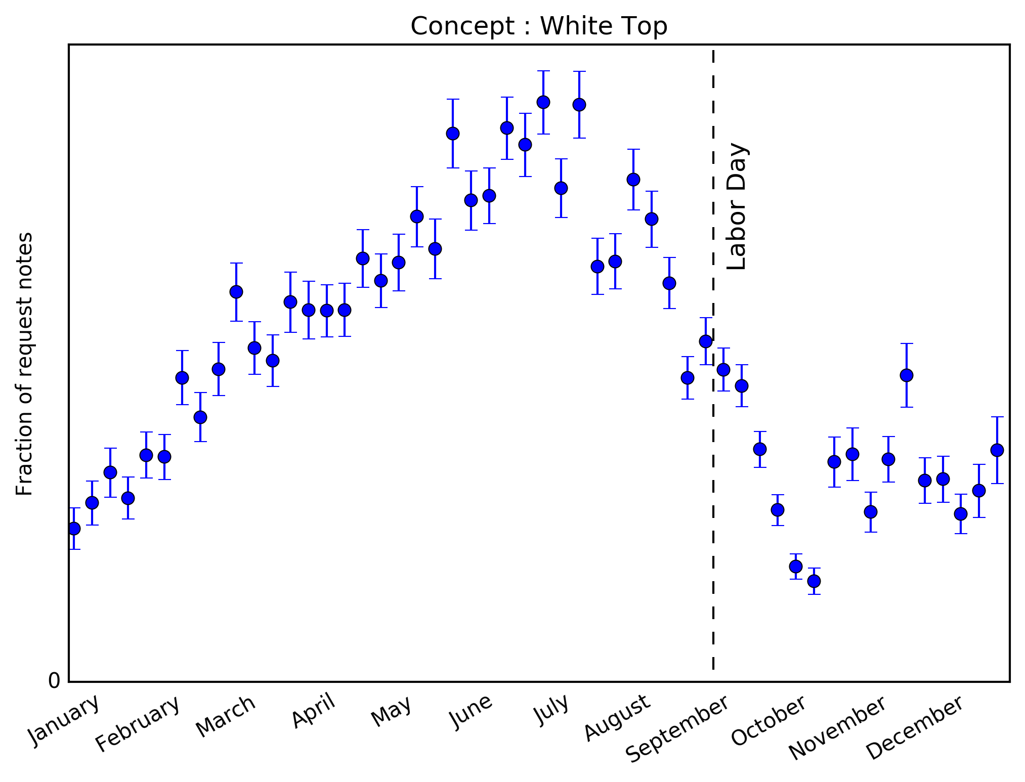
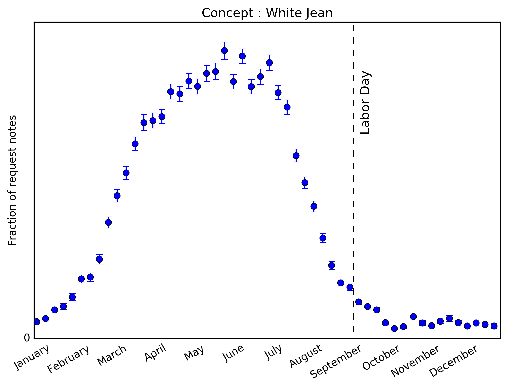
The time-series for requests within each topic are shown above with \(1\sigma\) confidence intervals. It seems clear that in both cases, our clients are requesting more white items before Labor Day than after. But it also looks like the demand for white tops drops by about 50% after Labor Day whereas the demand for white jeans goes down to about 10% of its maximum value. So it seems that clients are telling us that while they’re not interested in white bottoms after Labor Day, white tops are not as irrelevant. No sharp declines are seen.
Seasonal variability of probability of shipment
Since our company is specialized in personalization, we have the goal to match our client’s needs, even if it goes against conventional fashion wisdom. This is reflected in our inventory position at different times of the year, and also in the exceptional ability of our stylists to understand what our clients need.
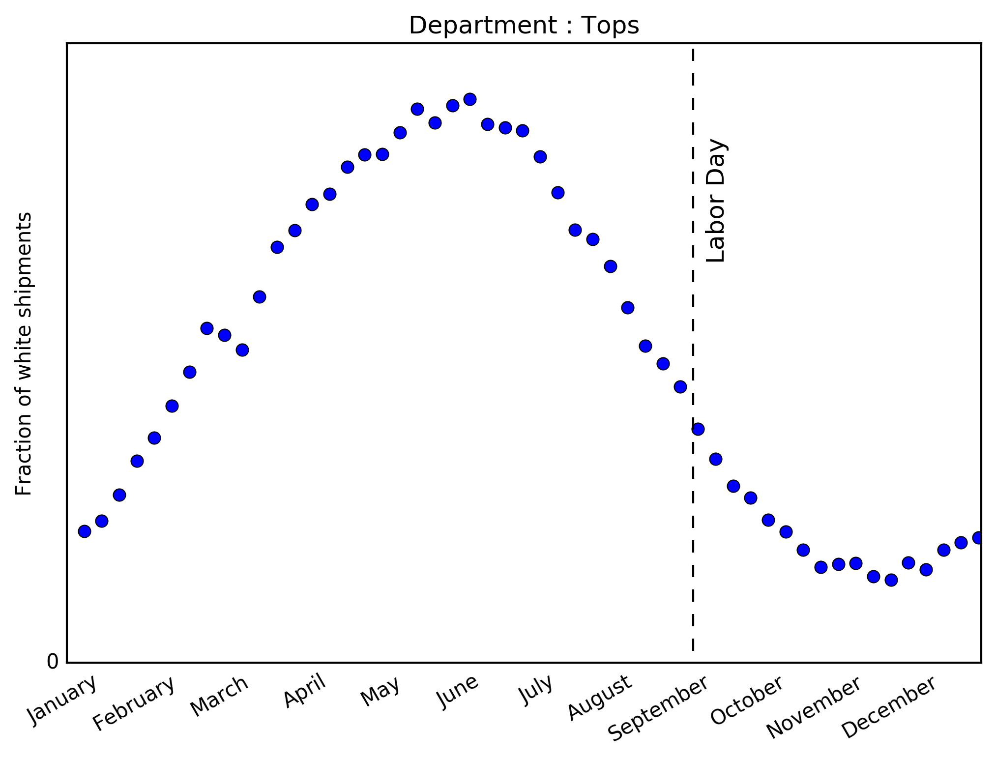
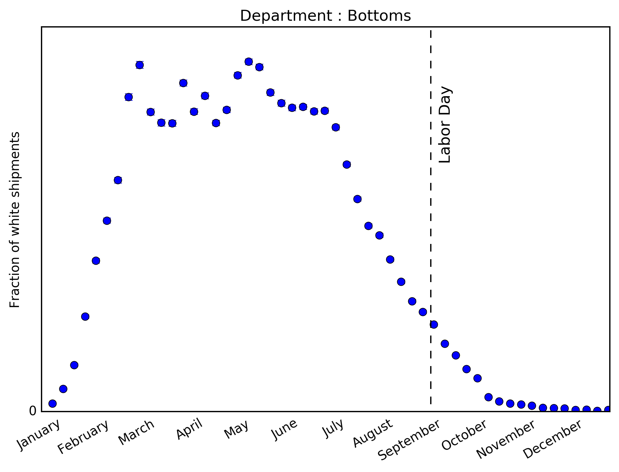
These panels now represent the weekly fraction of \(\textit{shipped}\) items that are white, within both tops and bottoms. The temporal trend in each category is impressively well-aligned with the request topic trends above. This not only corroborates the timing of white seasonality, but demonstrates Stich Fix’s focus on the client experience.
Seasonal variability of odds of purchase
We’ve shown how client requests change with time and how stylists react to them in terms of shipment volume. A final test is the client’s measured propensity to purchase the white apparel we send them. To answer that question, there are a few things we want to consider. A simple time-series of \(odds(white; time)\) falls short. Stitch Fix as a whole has week-to-week variability in such metrics, some due to internal decisions and some due to market fluctuations as whole.
There’s another important consideration as well. We have a lot of different styles in our inventory that are white, of varying popularity and depth. A clear source of bias in a model like this is which styles we’re sending at what times of year.
For example, imagine our buying team purchases white heavily in the summer, and doesn’t replenish. Good styles fly out the door like hotcakes, meaning there’s selection bias in which styles are left in inventory come September. In fact, the quantity of each style will decay exponentially, with a depletion rate proportional to the probability of purchase:
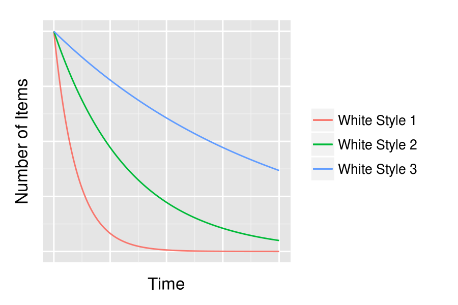
If we were to look at the odds of purchasing white at the beginning of the time window above versus the end, ignoring style distribution, it would look like preference for white was going down. But that would be a false conclusion, driven by the style mix.
To control for this, we’ll use a generalized linear model. In this model, \(\textit{white}\) is a boolean factor that is False for all other colors. We treat the week of year categorically, and express the odds of purchase by:
\[\log \Big( \frac{p}{1-p} \Big) \sim white + t_i + white*t_i + style\]where each observation is a boolean outcome representing the client’s decision to purchase an article of clothing we offered. Here, the \(\textit{white}\) term accounts for any overall difference in preference for white vs other colors, and the \(t_i\) term accounts for external fluctuation in company metrics. The regularized style categorical accounts for the quality of specific styles we may have at any point in time, flexible to varying amounts of data per style. The odds of purchase for any item will then be:
\[ odds \sim exp(white) * exp(t_i) * exp(white*t_i) * exp(style)\]Results from the last two years were modeled in R using mbest. Below we plot just the interaction \(\exp(white*t_i)\), with \(\pm 2\sigma\) standard errors on the interaction term only. The “relative” odds plotted are therefore relative to the remaining terms – the style, the time of year, and overall white preference.
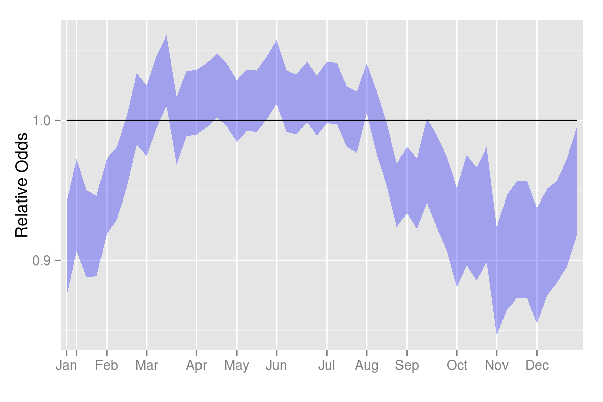
What we see is that there is, indeed, a relative preference for white in the summer months over the winter months. However, there is no step function in preference right at Labor Day in the beginning of September.
The Verdict: Reasonable trend
We conclude from these analyses that the axiom “No white after Labor Day” is simply using Labor Day as a symbolic end to the season, since white downtrends smoothly. We see requests & stylist preference for white bottoms drop sharply outside summer months, while white tops drop less fully. The odds of purchase of the white apparel we do send only drops about 10% from summer to winter. So, while white is more of a summer color than a winter color, the word No in the “No white after Labor Day” may be a fairly harsh edict given our observations of what people actually wish to buy. Stay tuned for our future trend reports!