Overview
We are excited to announce Diamond, an open-source Python solver for certain kinds of generalized linear models. This post covers the mathematics used by Diamond. The sister post covers the specifics of diamond. If you just want to use the package, check out the Github page.
Logistic Regression Using Convex Optimization
Many computational problems in data science and statistics can be cast as convex problems. There are many advantages to doing so:
- Convex problems have a unique global solution, i.e. there is one best answer
- There are well-known, efficient, and reliable algorithms for finding it
One ubiquitous example of a convex problem in data science is finding the coefficients of an \(L_2\)-regularized logistic regression model using maximum likelihood. In this post, we’ll talk about some basic algorithms for convex optimization, and discuss our attempts to make them scale up to the size of our models. Unlike many applications, the “scale” challenge we faced was not the number of observations, but the number of features in our datasets. First, let’s review the model we want to fit.
\(L_2-\)regularized logistic regression
Suppose we have observed \(N\) observations like \((x_i, y_i)\) where \(x_i\) is a p-vector of covariates for observation \(i\) and \(y_i\) is its binary outcome coded as 0/1. We wish to fit this model via maximum likelihood, which means
\[\max_{\beta} L(y | \beta) = \prod_{i=1}^N \textrm{Pr}(y_i=1 | \beta)^{y_i} (1 - \textrm{Pr}(y_i=1 | \beta))^{1 - y_i}\]where
\[\textrm{Pr} (y_i = 1 | \beta) = \frac{1}{1 + exp(-\beta^T x_i )}\]For convenience, we prefer to minimize the negative log-likelihood instead of equivalently maximizing the likelihood. Additionally, we’ll add an \(L_2\) penalty term, \(P\), which corresponds to a \(N(0, P^{-1})\) multivariate Gaussian prior on \(\beta\) (see derivation here). Therefore, we wish to find a \(\beta\) to minimize
\[\sum_{i=1}^N -y_i \textrm{log}~\textrm{Pr}(y_i=1) - (1 - y_i) \textrm{log}~(1 - \textrm{Pr}(y_i=1)) + \frac{1}{2}\beta^T P \beta\]We tried a few techniques to estimate \(\beta\), starting with the simplest.
Gradient descent
The first approach we tried was gradient descent. For the simplest version of gradient descent, all we need is to compute the derivative of the function we wish to minimize, and choose a step size, \(\gamma\). Then, at each iteration, we update according to this rule:
\[\beta_{t+1} = \beta_t - \gamma \nabla_t\]For our problem, the gradient is
\[\nabla_t = \sum\limits_{i=1}^N x_i (p_i - y_i) + P \beta_t\]Since our negative loglikelihood function is convex, under some mild conditions on \(\gamma\), this algorithm is guaranteed to converge to the global optimimum, eventually. Gradient descent is nice because it’s
- Simple. This means:
- easy to code!
- easy to test!
- easy to debug!
- General: works on a wide variety of problems
- A slight variant of this, stochastic gradient descent, scales to very, very large training data sets. However, our problem was scaling to a large number of features.
Unfortunately, we found gradient descent to be too slow for the number of parameters we wanted to estimate. So we tried another classic optimization algorithm, Newton’s Method.
Newton’s Method
You might remember this from undergraduate calculus, but if it’s been a while here’s a quick refresher.
Reminder of Newton’s method: Finding Zeros of a 1D Function
To illustrate Newton’s method, let’s start with a very simple problem: find an \(x\) such that \(f(x) = 0\). To do this, Newton’s method uses a linear approximation of \(f\) that goes like this.
- Choose an arbitrary starting point on the curve \(x_0\)
- Find the tangent to the curve at \(x_0\), and trace it down to the x axis
- Repeat the process with the new \(x\) value being the point where the tangent crossed the x-axis.
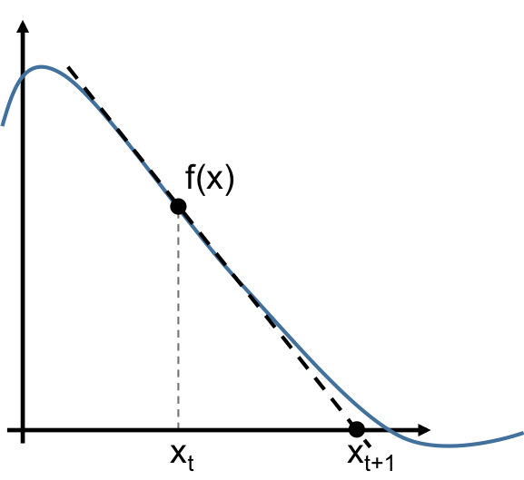
Mathematically, the update rule is
\[x_{t+1} = x_t - \frac{f(x_t)}{f'(x_t)}\]As with most iterative algorithms, we repeat this until the change,
\[|x_{t+1} - x_t| < \epsilon\]for some predefined tolerance parameter \(\epsilon\).
Simple optimization
What does this have to do with optimization, you ask? Well, for convex functions, we’re looking for the global minimum \(x^*\), and we know that \(f'(x^*) = 0\). So we can use the algorithm we just described not on \(f\), but on \(f'\), in order to find \(x^*\). Concretely, this means using a linear approximation to \(f'(x)\) at each iteration, and therefore a quadratic approximation to \(f(x)\).
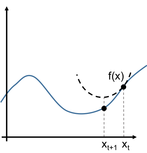
Mathematically, the update rule is
\[x_{t+1} = x_t - \frac{ f'(x_t) }{ f''(x_t) }\]Again, we repeat this iterative algorithm until some stopping condition is met. Common rules are
- \[|x_{t+1} - x_t| < \epsilon_x,\]
i.e. our parameter changes less than some predefined amount.
- \[|f(x_{t+1}) - f(x_t)| < \epsilon_f ,\]
i.e. our objective function changes less than some predefined amount.
- and stop after a set number of iterations, no matter what.
Newton’s method applied to logistic regression
In vector notation, one iteration of Newton’s method is
\[x_{t+1} = x_t - H^{-1}_t\nabla_t\]When we use Newton’s method to find the parameters of a logistic regression problem, we’re using an algorithm known as iteratively reweighted least squares (IRLS). R users will recognize this as the default method for fitting generalized linear models in glm. Unfortunately, inverting the Hessian matrix at every iteration does not scale well with the number of parameters, so we also found this method inadequate in its simplest form. However, with a couple of tricks, we were able to make it work. These tricks came from this paper by Thomas Minka, to which we are greatly indebted.
Fixed-Hessian
It’s possible to compute and invert the Hessian once, and then use it in place of the true Hessian at every iteration. Let’s call our approximate Hessian \(\tilde H\). As long as \(H - \tilde H\) is positive definite, this is guaranteed to converge (see Minka’s paper for a proof). For an arbitrary penalty matrix \(P\), a good choice is
\[\tilde H = -\frac{1}{4} X X^T - P\]This leads to the following update rule:
\[\beta_{t+1} = \beta_t - \tilde H^{-1}\nabla_t\]Conjugate gradient trick
In practice, it’s faster to take \(u = -\tilde H^{-1}\nabla\) as a step direction, and then use the conjugate gradient method to determine a step size \(\gamma\). Mathematically, our update rule will be
\[u = \tilde H^{-1}\nabla\] \[\beta_t = \beta_{t-1} - \gamma u\]where \(\gamma \in \mathbb{R}\). To determine how large of a step we should take, consider the second-order Taylor expansion of our penalized, negative log-likelihood function \(f\) around a point \(\beta_0\):
\[f(\beta) \approx f(\beta_0) + \nabla_0^T(\beta - \beta_0) + \frac{1}{2}(\beta - \beta_0)^TH_0(\beta - \beta_0)\]Now, let’s optimize this function with respect to our step size \(\gamma\) by taking its derivative, setting it equal to zero, and solving.
\[\frac{\partial f}{\partial \gamma} = (\nabla f(\beta))^T (-u)\] \[\frac{\partial f}{\partial \gamma} = (H_0\beta + \nabla_0 - H_0\beta_0)^T(-u)\] \[\frac{\partial f}{\partial \gamma} = (H_0(\beta_0 - \gamma u) + \nabla_0 - H_0\beta_0)^T(-u)\] \[\frac{\partial f}{\partial \gamma} = (- \gamma H_0 u + \nabla_0)^T(-u)\]Now, set equal to 0 and solve for \(\gamma\). Note that H is symmetric, so \(H^T = H\)
\[0 = (- \gamma H_0 u + \nabla_0)^T(-u)\] \[0 = \gamma u^T H_0^T u - \nabla_0^T u\] \[\gamma = \frac{\nabla_0^T u}{u^T H_0 u}\]Since H is positive definite, this is a minimum of f in the neighborhood of \(\beta_0\), which is what we want, since we are minimizing the negative, penalized log-likelihood.
Mixed-effects models
An important class of this kind of model is mixed effects (see part II). In this case, the key idea is that we can almost separate the optimization problem across levels of the random effects. But the fixed effects are common to the model for each level, so we can’t really separate the problem. This does, however, suggest a strategy that alternates between two stages:
- solve for fixed effects coefficients
- solve for random effects coefficients with the fixed effects from (1) treated as constants
Because the whole problem is convex, this alternating iteration will converge to the global optimum. This is numerically possible because we can store the Hessian as a sparse, block diagonal matrix and thus afford to invert it. This lets us use the quasi-Newton method described above. With this methodology, we can fit models with millions of random effect levels. In principle, one could also separate the problem in (2) across levels and solve them in parallel, potentially making it faster still.
Conclusion
With these two tricks, we have written a very fast, Newton-inspired, implementation of this algorithm in Python 2.7 for logistic (binary outcome) and cumulative logistic (ordinal outcome) regression with very general \(L_2\) regularization. Our use case is mixed-effects models with tens of thousands of parameters. Our implementation is called diamond, and we are going to open-source it soon. Stay tuned!
Sources
- Boyd and Vandenberghe’s book is a wonderful reference on convex optimization
- Minka provided the necessary tweaks to make Newton’s method work for this particular problem
- Thanks to Brad Klingenberg, PhD for mentorship on this project