Introduction
At Stitch Fix, like many businesses, we pay close attention to the probability that a client who visits the site will sign up for the service (aka the “conversion rate”) to understand how visitors interact with the site and look for ways we can do better.
We can frame conversion prediction as a binary classification problem, with outcome “1” when the visitor converts, and outcome “0” when they do not. Suppose we build a model to predict conversion using site visitor features. Some examples of relevant features are: time of day, geographical features based on a visitor’s IP address, their device type, such as “iPhone”, and features extracted from paid ads the visitor interacted with online.
A static classification model, such as logistic regression, assumes the influence of all features is stable over time, in other words, the coefficients in the model are constants. For many applications, this assumption is reasonable—we wouldn’t expect huge variations in the effect of a visitor’s device type. In other situations, we may want to allow for coefficients that change over time—as we better optimize our paid ad channel, we expect features extracted from ad interactions to be more influential in our prediction model.
In this post we’ll take a look at how we can model classification prediction with non-constant, time-varying coefficients. There are many ways to deal with time dependence, including Bayesian dynamic models (aka “state space” models), and random effects models. Each type of model captures the time dependence from a different angle. In this post we will keep things simple and look at time-varying logistic regression that is defined with a regularization framework. We found this to be quite intuitive, easy to implement, and have observed good performance using this model.
Notation and Intuition
We first introduce the following notation:
- \(Y_t\) is the response at time \(t\). In conversion classification, we have a 1 or 0 response—the visitor at time \(t\) did or did not convert.
- \(X_t\) are the features at time \(t\).
- \(P_t\) is the probability of a response \(Y_t = 1\) at time \(t\).
- \(B_t\) is the coefficient matrix at time \(t\).
Recall that in a static model, we assume \(Y_t = f(X_t)\), where \(f\) does not depend on \(t\). In contrast, in time-varying models we assume that the relationship between features and responses varies over time: \(Y_t = f_t(X_t)\). Additionally, we expect that \(f_t\) and \(f_{t+1}\) differ very little unless a “change-point” occurs.
Using a regularization framework, we will detect these change-points and shrink noise to zero by penalizing the differences between \(f_t\) and \(f_{t+1}\). With different choices of penalty functions we can encode different “time dynamics” which describe how the coefficients evolve over time.
Time-varying models within a regularization framework have previously been used to tackle problems in disease progression modeling1, economic research2 and dynamic networks in social and biological studies3, 4, to name a few. As data scientists in a fast-growing company, we find time-varying models to be useful for understanding the progression of customer behaviors.
In the rest of this post, we’ll introduce the time-varying model more formally, discuss its implementation via reparametrization, and demonstrate its power with an illustrative example.
The Time-Varying Model
The mathematical formulation of a time-varying model that we use is based on existing regularization frameworks. For interested readers who are not familiar with these frameworks, we refer to the listed references for continued reading.
Formulated under a regularization framework, our target is to optimize the parameters with respect to the objective function
\[\sum_t L(B_t|X_t,Y_t) + \sum_{t \ge 2} P(B_t - B_{t-1}),\]where \(L(Y_t,B_tX_t)\) is the log likelihood of the target model and \(P(B_t - B_{t-1})\) is the penalty of the difference between \(B_t\) and \(B_{t-1}\). In our example of modeling conversion rate, we would specify \(L(Y_t,B_tX_t)\) to be the log-likelihood function for logistic regression.
An additional penalty \(\sum_t P(B_t)\) could also be added onto the objective function for simultaneous feature selection, but for simplicity, we will not discuss it here.
In the objective function, differences between coefficient matrices at time \(t-1\) and \(t\) are penalized, so that small perturbations between \(B_{t-1}\) and \(B_t\) will be treated as noise and shrink towards zero, whereas signals and big jumps will be detected.
Implementation with Reparametrization
One of the nice things about this regularization framework for time-varying models is that we can reparametrize \(B_t\) to recover a static model. Setting \(\delta_1 = B_1\) and \(\delta_t = B_t - B_{t-1}\) for \(t \ge 2\), we see that \(B_t = \sum_{k \le t} \delta_k\) and can rewrite our objective function as
\[\sum_t L(Y_t,B_tX_t) + \sum_{t \ge 2} P(B_t - B_{t-1}) = \sum_t L(Y_t; \delta_1, \dots, \delta_t) + \sum_{t \ge 2} P(\delta_t).\]One can then use existing R packages for penalized likelihood, for example library(glmnet) and library(ncvreg), to implement the time-varying models.
Choice of Penalty
In this framework, the specific form of the penalty function \(P\) needs to be specified. Different choices of \(P\) allow modelers to encode different beliefs about the dynamic patterns of the coefficients. Some useful penalty functions are presented here, along with their corresponding evolutionary patterns.
- Setting \(P(B_t - B_{t-1})\) as MCP5, SCAD6, or LASSO7 encodes the pattern that only a few coefficients change at a time. These penalties are best used in cases where we expect only a handful of coefficients to change at a time.
- Setting \(P(B_t - B_{t-1})\) as Ridge8 encodes smooth transitions from time \(t-1\) to \(t\).
- Setting \(P(B_t - B_{t-1})\) as GROUP LASSO8 causes the coefficient matrix to globally restructure at a select few change-points, so that coefficients remain piecewise constant outside of these change-points.
Which penalty should we use if we don’t have a prior understanding of the evolutionary pattern of the coefficients? In this case, we recommend using non-convex penalties, such as MCP or SCAD. This recommendation is based on the fact that the more popular LASSO penalties can be biased when data is noisy or when we have some co-linearity, such as when there are many time-dependent settings.
An Illustrative Example
To wrap up this post, we consider a simple longitudinal classification problem with \(N = 300\) observations at each of \(T = 15\) timepoints. At each time \(t\), we independently sampled 30 features \(X_t\) from a standard normal distribution. Thus the true coefficient matrix \(B = (B_1, \dots, B_T)\) is of size \(30 \times 15\). We set each entry \(B_{ij}\) to be small random noise around zero for \(j = 1\) to \(j = 27\) and the remaining three vectors of time-varying coefficients to be piecewise constant, as shown in the first figure in the image below. We generated the binary outcome vectors \(Y_t\) so that each entry is 1 with probability \(p_t\) following \(\text{logit}(p_t) = X_t B_t\).
With the generated data, we estimated the coefficients with time-varying models using the Ridge, LASSO, and MCP penalties. We benchmarked these results against the results using static logistic regressions (one trained at each time \(t\), and one trained on the whole data). Results from all methods are shown below.
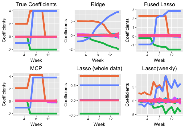
As shown, the time-varying model with non-convex penalty MCP has the best estimation accuracy and change-point detection. Fused Lasso, which is the time-varying model with LASSO penalty, has larger errors, as expected and discussed in the previous section. The time-varying model with the Ridge penalty yields estimates with smooth transitions, which are often desired in real applications for better interpretability. Compared with the time-varying models, the static models perform worse because the time-varying effect is not estimated, or noise is too easily detected.
We have found these time-varying models to be very useful for our classification tasks and hope it will help you with your data analysis and research also!