Word Tensors
To see the first part of this article, check out “Stop Using word2vec”
In the previous post, we saw that we can get word vectors by factorizing a 2D matrix of word co-occurrences. But what do we get if we factorize a 3D tensor?
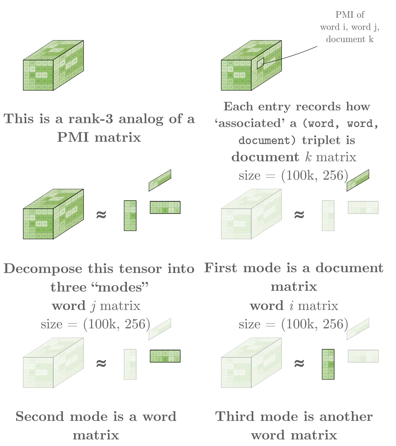
If our tensor is the association between word X, word Y within document Z, it turns out that like doc2vec, we can get word and document vectors!
In skipgram matrix factorization, we SVD factorize a matrix like:

This says: construct a large, potentially very sparse, matrix M where we’ve counted how frequently word x cooccurrs near word y and normalized that count to get the probability p(x, y). Then we divide by the probabilty of each word by itself (instead of the cooccurrence), where p(x) and p(y) are essentially the popularity of word x and word y. If this ratio is far above or below 1.0, then there’s something special about the relationship between token x and y, but if it’s near 1.0, then they co-occcur at the ‘usual’ rate. The log of this ratio is called the pointwise mutual information and has deep connections to information theory. Read our previous blog post “Stop Using Word2vec” for more details.
But in tensor factorization we can choose to factorize a tensor like this:

This is similar to the previous matrix, but with that extra dependence on z this tensor is now indexed by three variables instead of two. And like in the 2D case, we measure how often the three objects x, y, z cooccur (instead of just x and y) and then divide by p(x), p(y) and p(z) that measure the individual word probabilities. In this example, we’ll count how frequently word x cooccurs near word y in document z. At Stitch Fix, z is an index over all comments about a single piece of clothing, so z typically encodes all written information about a particular style or item of clothing.
Having formed this large 3D tensor, we can then decompose it into three 2D modes: one mode for the word index x, one mode for the word index y, and another for document index z.

In this example, the first and second modes contain word vectors, which are word representations our clients use to describe their fixes. The third mode represents document vectors which yields a summary about everything said about one style.
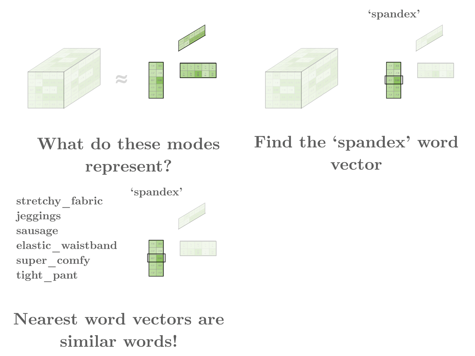
 Interpreting these matrices is easy. Out of one of the two word matrices, we can extract the row vector corresponding to the word
 spandex and see what other row vectors are similar. And voilà! spandex turns out to be similar to stretchy_fabric and jeggings. Just like the original word2vec, we get that these tokens are similar because they cooccur in similar contexts. Spandex on occasion can squeeze your body into awkward ways, which explains why the token sausage ends up in similar contexts.
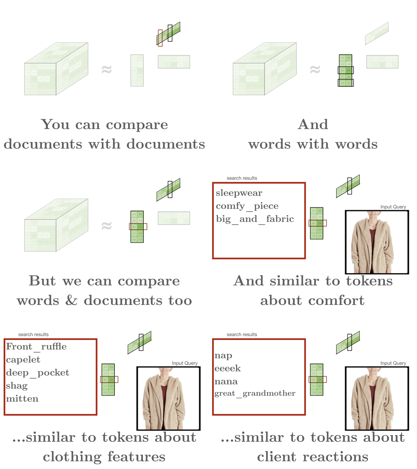
 Our documents are composed of all comments written about a single style. So if we look at what is similar to a denim jacket, the results are populated with sensible items: denim jackets, jackets with similar cuts, and jackets with similarly prominent brass buttons. If our input query is a salmon-colored Dolman top, the closest items are other Dolman tops with varying colors.
 We aren’t limited to exploring vectors within a single mode – we can compare vectors from words matrices to vectors within the document matrix. This cross-modality allows us to find interesting relationships between styles and their descriptions. For one of our most snuggle-worthy styles, we can see that it’s closest word vector is
 cocoon_cardigan!
Tensor Decomposition
There’s only three steps to computing word tensors. Counting word-word-document skipgrams, normalizing those counts to form the PMI-like M tensor and then factorizing M into smaller matrices.
But to actually perform the factorization we’ll need to generalize the SVD to higher rank tensors 1. Unfortunately, tensor algebra libraries aren’t very common 2. We’ve written one for non-negative sparse tensor factorization, but because the PMI can be both positive and negative it isn’t applicable here. Instead, for this application I’d recommend HOSVD as implemented in scikit-tensor. I’ve also heard good things about tensorly.
Conclusion
Counting and tensor decompositions are elegant and straightforward techniques. But these methods are grossly underepresented in business contexts. In this post we factorized an example made up of word skipgrams occurring within documents to arrive at word and document vectors simultaneously. This kind of analysis is effective, simple, and yields powerful concepts.
Look to your own data, and before throwing black-box deep learning machines at them, try out tensor factorizations!
