On the Stitch Fix Algorithms team, we’ve always been in awe of what professional stylists are able to do, especially when it comes to knowing a customer’s size on sight. It’s a magical experience to walk into a suit shop, have the professional shopping assistant look you over and without taking a measurement say, “you’re probably a 38, let’s try this one,” and pull out a perfect-fitting jacket. While this sort of experience has been impossible with traditional eCommerce, at Stitch Fix we’re making it a reality.

Sizes set by apparel manufacturers are arbitrary. There is no industry standard for what constitutes a small shirt, and the dimensions used by different manufacturers can vary widely. Since manufacturers aren’t consistent, people’s judgments of their own sizes can be inconsistent. This means we have two problems when choosing clothes to fit our clients: 1) We’re not sure what size our items are, and 2) we’re not sure what size our clients are. Fortunately, we do receive rich customer feedback every time a customer checks out.

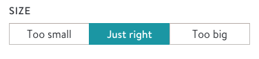
Every time a client checks out, he or she rates whether each item was too big, too small, or just right. This provides a hint about the true size of both the client and the item at the same time, though it’s up to us to figure out which is which. If a client rates an item too big, that could mean:

1. The item was bigger than we thought,
2. The client prefers a smaller size than we thought, or
3. Both of the above are true.^[1]

At Stitch Fix, we have put in place a principled modeling approach to determine the true meaning of clients’ feedback and match client sizes to merchandise sizes. Inspiration for our solution came from a surprising place: The origins of the SAT college placement test.

Item Response Theory: The Original Recommendation System

In 1947, the Educational Testing Service (ETS) was founded to administer nationwide standardized tests, most notably the SAT and GRE. ETS needed to continuously create new versions of the test with new problems so that students would not be tempted to memorize solutions from previous versions. Not only does the test change over time, but individual students receive different versions of the test, so that there’s no use peeking at a neighbor’s answers during the test. This creates a problem for grading: If each student sees a different set of problems, how can grades be fairly compared? One student might receive a test filled with easy questions and get a high score, while another equally bright student might receive mostly difficult questions and get a low score. Perhaps the solution is to weight the questions by difficulty, but in that case how can the difficulty of new questions be assessed?

Researchers at ETS derived a solution that became known as Item Response Theory, or IRT.^[2] IRT makes the assumption that students lie on a continuum of competency, which ultimately corresponds to a score on the test. Question difficulty is projected onto the same continuum. Students should be more likely to answer a given question correctly if they are more competent than the question is hard, and vice versa.

At Stitch Fix, we’ve used IRT to determine the difficulty of stylist judgments while also rating stylist competence, as discussed in a previous blog post. For the simple IRT model described there (also known as a Rasch model), to assess test scores we fit an ability parameter, \(\eta_{s}\), for each student \(s\) and a difficulty parameter, \(\eta_{q}\), for each question \(q\). We can then model the probability of student \(s\) providing a correct response to question \(q\) as

This results in an item characteristic curve in which the difference between ability and difficulty (\(\eta_{s}-\eta_{q}\) in the above equation) implies the likelihood of answering the question correctly, depicted in the figure below:

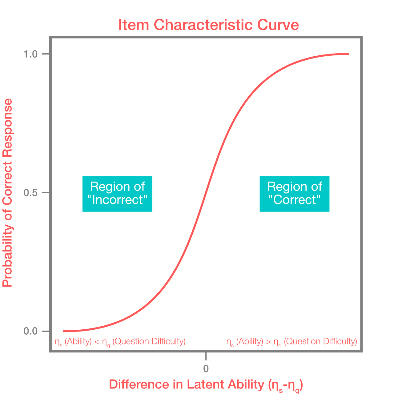
The item characteristic curve provides a likelihood for a given data set of responses conditioned on a set of choices for parameters \(\eta_{s}, \eta_{q}\). Given a set of test scores, we can solve for the best set of parameters using maximum likelihood estimation techniques.

Solving the Catch-22 with IRT

As it turns out, the problem of fit can be framed similarly to the test question problem. Like SAT questions, we can assume that each item lies on a continuum of sizes. The same goes for our clients. You can think of this like filling in the gaps on numeric dress sizes: Clients might say they’re a dress size 2, 4, 6, 8, etc., but we can assign them an even more nuanced size, say 2.4. We can do the same for the dresses themselves.

The math works almost exactly the same way for size as it does for SAT questions, with one key difference. On a test, students get answers wrong or right, and that’s what we use to judge whether they are smarter than the question or vice versa. With clothes, we get three possible response values: too small, too large, or just right. We can solve this using an ordinal logistic likelihood function. We fit two classifiers simultaneously: One classifier for too small vs. just right, and one for just right vs. too large. In the IRT literature, this framing is known as the polytomous Rasch Model. We update the IRT equation with outcome \(X\) indicating the size rating (too small, just right, or too large), and \(\tau_k\) as the threshold for size response \(k\), over clients \(c\) and items \(i\)^[3]:

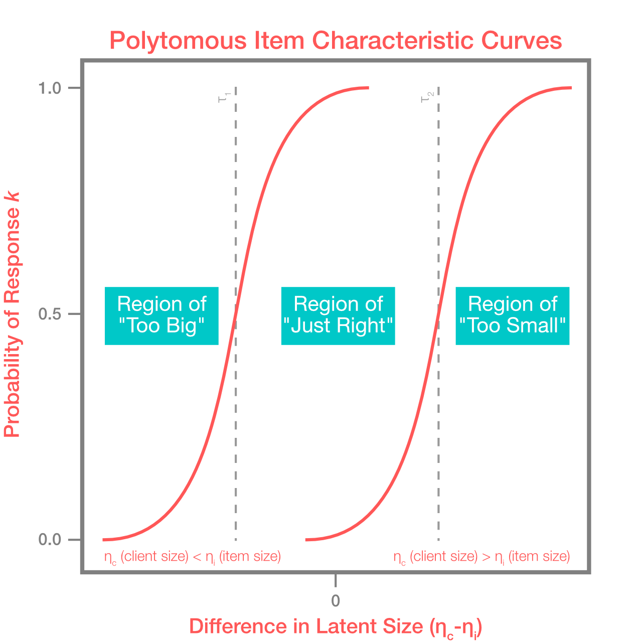
This is illustrated in the figure below. When the size difference is highly negative (client sizes much smaller than item sizes), the too large response is most likely. As we increase this metric, just right responding increases and ultimately becomes the dominant response when the difference is close to zero. Continuing to move up, highly positive differences are associated with the too small response becoming most common. This is similar to the item characteristic curve above, just expanded to the case of more possible responses.

Once we realized that this might work, we quickly hacked together a prototype in Stan^[4]. Stan is a language for specifying probabilistic models, and thankfully it is forgiving enough to allow us to easily swap out an ordinal logistic outcome variable in place of the usual binary. The code in Stan is surprisingly simple, as you can see in the Appendix. Our most common size was medium, so we picked a few thousand medium items that had been sent to the most clients. This resulted in a set of modeled latent sizes \(\eta_{c}\) for each of the clients, and a separate set of latent sizes \(\eta_{i}\) for each of the items in inventory.

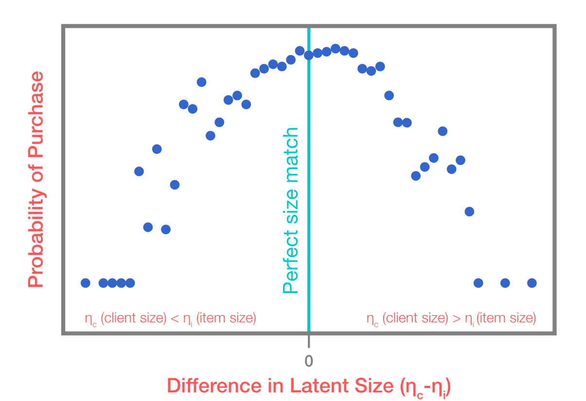
To validate our model, we looked at how predicted size related to the success rate of items sent, that is, the likelihood the client would purchase an item if it was included in the fix. Predicted size can be thought of as the \(\eta_{c}-\eta_{i}\) in the example above. The results are displayed in the figure below. Clients who were a good match for the items they were sent, as measured by a low absolute value for \(\eta_{c}-\eta_{i}\) according to the model, had the highest success rate. Success rate falls off as the difference becomes larger in either direction. Note that success rate itself was not used to fit the model, only client feedback!

Solving the Cold Start Problem

New users can be tricky for recommender systems. The model above was trained on clients’ historic feedback for individual clients and items. What do we do about clients who recently signed up and have no past history on the service? Since IRT is structurally a regression model, it is easy to add coefficients for client size, manufacturer, or whatever other attributes we find important. For example, if we know Nike sneakers tend to run small, the model can help us learn that, and we’ll assume new pairs of Nikes will run small until the data tells us otherwise. This approach serves to quantify knowledge that professional stylists have traditionally held in their brains.

Random Effects All the Way Down

One tricky aspect of IRT is fitting; traditional methods can be difficult to scale to millions of clients and items. However, as we’ve alluded, IRT is regression-like in its formulation. It turns out that simple versions of IRT form a special case of a much more general class of models we find useful at Stitch Fix – generalized mixed effects models. In these models, we selectively regularize some terms (e.g. the latent sizes of clients).  We’ve invested greatly in learning how to fit generalized mixed effects models reliably at scale, so casting IRT into this framework makes it much easier to productionize.

Let’s write out some math for classical IRT just to be more specific.

First we model the outcome, whether or not a student correctly answers a question, as

This says that the log odds of the probability of a correct response for question \(q\) from student \(s\) is modeled by some overall mean, along with contributions for the difficulty of the question (\(\eta_q\)) and question-answering ability of the student (\(\eta_s\)).  

As we’ve written it, the model in equation (1) is a perfectly valid generalized linear model. But if we have thousands of students and questions, and sometimes very few observations per student or question, we risk overfitting if we don’t regularize estimates for \(\eta_q\) and \(\eta_s\). Mixed effects modeling (and classical IRT) adds an assumption of the distribution of the parameters \(\eta_q\) and \(\eta_s\). If we model questions’ difficulties and students’ abilities as Gaussians, we can write:

We’ve added distributions for the \(\eta_s\) and \(\eta_q\), introducing parameters \(\sigma^2_Q\) and \(\sigma^2_S\), the learned variances of our questions and students’ abilities.  

Now it’s easy to see how similar IRT is to our sizing problem. We can use an ordinal logistic model and write:

We’ve just switched out our binary outcome for an ordinal, and our student and question random effects for client and SKU.  

From here it’s easy to include terms for the sizes a client signs up as, or the sizes of the items he or she has rated. Then the random effects only have to account for the deviation of a client’s true size away from his or her signup size. This way, we can start a client out at the true size implied by his or her signup information, and then slowly learn over time, as he or she rates many of our items, what his or her true size is. Each item we send to a client serves as a “measuring stick,” allowing us to zero in on his or her size and get it just right.

LME4 in R or MixedModels(also from Doug Bates) let you easily specify and write these models. Stan, PyMC3, and edward are great tools for more flexible modeling.  

Conclusion

There’s so much about traditional retail that has been difficult to replicate online. In some senses, perfect fit may be the final frontier for eCommerce. Since at Stitch Fix we’ve burned our boats and committed to deliver 100% of our merchandise with recommendations, solving this problem isn’t optional for us. Fortunately, thanks to all the data our clients have shared with us, we’re able to stand on the shoulders of giants and apply a 50-year-old recommendation algorithm to the problem of clothes sizing. Modern implementations of random effects models enable us to scale our system to millions of clients. Ultimately our goal is to go beyond a uni-dimensional concept of size to a multi-dimensional understanding of fit, recognizing that each body is unique. We’re hard at work on the next stage. Watch this space for updates!

Appendix

Stan code for model:

data {
    int<lower=1> J;
    int<lower=1> K;
    int<lower=1> N;
    int<lower=1,upper=J> jj[N];
    int<lower=1,upper=K> kk[N];
    int<lower=1,upper=3> y[N];
}

parameters {
    real delta;    
    real alpha[J];
    real beta[K];  
    ordered[2] c;
}

model {
    alpha ~ normal(0, 1);
    beta ~ normal(0, 1);
    delta ~ normal(.75, 1);
    for (n in 1:N)
        y[n] ~ ordered_logistic(alpha[jj[n]] - beta[kk[n]] + delta, c);
}