As Mark Twain may have said: “Prediction is very difficult, especially about the future” [1]. Alas, at Stitch Fix we do this all the time. Specifically, we need to predict upcoming demand for our inventory. This allows us to determine which clothes to stock, so we can order the correct number of units for each item, and to allocate those units to the right warehouses, allowing us to deliver delightful fixes for our clients!
As the year unfolds, our demand fluctuates. Two big drivers of that fluctuation are seasonality and holidays. With the holiday season upon us, it’s a great time to describe how both seasonality and holiday effects can be estimated, and how you can use this formulation in a predictive time series model.
In this post, we describe the difference between seasonality and holiday effects, posit a general Bayesian Holiday Model, and show how that model performs on some Google Trends data.
If you want to skip to the examples, click here.
Seasonality vs Holidays
For the purpose of this post, we are using the term “holiday” to denote an important yearly date that affects your data observations. This usually means days like Christmas and New Year’s Eve, but it could also refer to dates like the Superbowl, the first day of school, or when hunting season starts.
Holidays are in contrast to “seasonality,” which is a longer term effect that can persist over multiple weeks or months. We will see that both contribute to our data observations, and distinguishing between them is important when we want to make decisions based on the outcome of our model.
Holiday effects show up in many different sorts of time series, including retail sales [2, 3, 4], electrical load [5], social media events [6], along with many others.
Unfortunately, holiday effect data is sparse, since most holidays occur only once a year. Furthermore, many holidays are entwined within certain “seasonal” time periods. This makes modeling the effect especially difficult.
Most people think of holiday impacts as a spike in time, but this isn’t always the case. For example: in many retail stores across the globe, the entire month leading up to Christmas means increased sales. So we would want a holiday effect to reflect this ramp up. Conversely, if you are modeling the number of customers who will visit your brunch spot in late March/early April, you would expect a spike right on Easter Sunday. We would also want our model to reflect this phenomenon. If we are interested in demand for big screen T.V.s at our electronics store, we would expect a drop-off in sales after Super Bowl Sunday. Each of these examples lead to very different holiday effect profiles. Therefore, we want a model that is flexible enough to cover these cases (and many others!).
To robustly capture holiday effects within time series data, a model should meet several criteria:
- Flexibility in general shape: Holiday effects may suddenly spike, then disappear, or they may have long ascent/descent effects or sustained elevation over time.
- The effect of the holiday can be positive or negative.
- Discovery of peak location: Holiday effects may peak close to, but not exactly on, a holiday date.
- Sparsity: Holiday effects should be used sparingly, so as not to explain too much variation in the data.
Standard strategies for modeling holidays incorporate them as additive components into a model, and focus on the use of indicator variables for each holiday [6, 7]. This strategy places a “yes” on holiday dates and a “no” on the other days, “indicating” which dates are active. To do this, one has to know all of the holiday dates on which to place a “yes.” The dates must include each occurrence of the holiday going back in time over all of the training data, and going forward, over the dates you wish to forecast against. An extension to this idea is having additional indicator variables within a user-specified range of dates before or after the holiday [2,4,5]. However, if the holiday effect is long-lasting, growth in the number of indicator variables can lead the model to overfit, especially when the data is sparse.
Below, we outline an approach that simultaneously minimizes overfitting with holidays, while also allowing for determining the contribution of individual holidays to the overall effect of the time series.
Being able to extract the contribution of each holiday to the observations is important when we want to make decisions based on the outcome of the model. Marketing teams would love to know that an increase in sales is due to Christmas coming up, and not due to Thanksgiving having passed, allowing them to run promotions targeting the correct holiday.
Bayesian Holiday Modeling
We begin with a list of holidays provided by the user (denoted the holiday calendar). These are the dates that one expects will influence the time series. For example, if you are a CPA, then you would expect your workload to increase after tax day (April 15th in the United States) so you would have April 15 in your holiday calendar. Retail marketers, on the other hand, would not necessarily have that date in their holiday calendar, but they might have the date that kids go back to school.
To generate a flexible model that encompasses all of the criteria above, we borrow from the space of probability distributions: We utilize an unnormalized skew-normal distribution function (where we approximate the normal CDF with an inverse logit). Probability distributions are not typically viewed as “functions” for typical regressions, but we find their flexibility in conforming to parameters exactly what we need for modeling holidays.
The effect from an individual holiday is modeled as a function of the difference between the date of the observation, and the closest date of that holiday. For example, if only Christmas and Easter are included in your holiday calendar, then the observation on February 12 would have holiday features [-49, 60], since it is 49 days (previous) since the nearest Christmas, and 60 days until the nearest Easter. The holiday effect for February 12 would then be a function of these features.
If there are \(H\) holidays considered in the model, then each observation has \(H\) holiday features as input to the model (\(H=2\) in the above example).
The Holiday Effect Function
Generating a model that encompasses all of the criteria we outlined above involves combining a lot of ingredients.
Our holiday effect function \(h(t)\) describes the effect of the holiday at date \(t\) as:
with
where
- \(\mu\) is the location parameter - it denotes how “offset” the effect is from the actual holiday date
- \(\sigma\) is the scale parameter - it denotes how broad the effect of the holiday is over time
- \(\omega\) is the shape parameter - it denotes how “peaky” the effect is in time
- \(\kappa\) is the skew parameter - it denotes how asymmetrical the holiday effect is around \(\mu\)
- \(\lambda\) is the intensity parameter - this denotes the magnitude of the holiday effect.
To get a feel for the types of effects able to be modeled, play with the sliders below to generate possible ranges from the Holiday Effect Function.
As the sliders show, our holiday effect function allows for extreme flexibility in both shape and location.
Two examples for the model are included for illustrative purposes. When pressing the “Santa Claus” button, we see a holiday effect corresponding to the ramp-up of searches for “Santa Claus” in Google Trends data. The effect starts to ramp about 7 days before Christmas, reaching its peak on the evening of the 24th of December, then abruptly crashing after the holiday.
The “Tax Return” example shows the effect of searches for “Tax Return” in Google Trends data. Searches do not begin until after April 15th (Tax Day in the United States) and slowly taper off throughout April and into early May.
Priors
Typically, we embed the holiday effect function within a larger model, like as a component for the mean of a count distribution. Using strict priors on the relatively few parameters, the function is able to express a wide variety of holiday effects without overfitting.
Setting priors for the parameters of the holiday effect function is done similarly to other Bayesian workflows [8]: Prior predictive checks should be completed to determine relevant scales and default values.
For the parameters in the model, the distributions chosen were:
- \(\mu \sim \mathcal{N}\left(0, \sigma_{\mu}\right)\).
- \(\sigma \sim \textrm{Gamma}\left(k_{\sigma}, \theta_{\sigma}\right)\).
- \(\omega \sim \textrm{Gamma}\left(k_{\omega},\theta_{\omega}\right)\).
- \(\kappa \sim \mathcal{N}\left(0, \sigma_{\kappa}\right)\).
- \(\lambda\) is drawn from a regularized horseshoe [9]
Setting the prior mean for \(\mu\) at zero implies we expect the effect to peak on the official holiday date. The standard deviation for the location, \(\sigma_{\mu},\) should be chosen such that each holiday doesn’t drift too far away from its original location. The coefficients of \(\sigma\) are chosen such that the locality of each holiday is controlled; preventing the effects of one holiday from exceeding the dates of its closest holiday neighbors. The scale and skew can be tuned to implement beliefs in how the effect of the holiday persists about the holiday date. Of course, using weakly informative priors here is a good alternative strategy if no prior information about your data are known (but this is rarely the case!).
The regularized horseshoe prior [9] for \(\lambda\) can be considered as a continuous extension of the spike-and-slab prior. This is a way of merging a prior at zero (the “spike”) with a prior away from zero (the “slab”), and letting the model decide if the coefficient should have a non-zero posterior. This encourages sparsity and resists using holidays to explain minor variation in the data.
Regularized Horseshoe
The coefficient for the intensity of each holiday (the \(\lambda\) parameter) is determined by the following prior:
where \(h_0\) is the expected number of active holidays, and \(H\) is the total number of unique holidays in the holiday calendar.
The prior on \(c^2\) translates to a Student-\(t_{\nu}\left(0, s^2\right)\) slab for the coefficients far from zero. We choose \(s = 3\) and \(\nu = 25\) and are typically good default choices for a weakly informative prior [9].
Having this prior on the holiday intensity is imperative for the model to work at all. Having no sparsity-preserving prior leads to each holiday being activated to overfit the observed data. Enforcing regularization via the horseshoe allows for realistic intensity values to be inferred from the data.
Immediate extensions to the model would be to have correlated structure among the holiday intensities, that would allow for prior beliefs of how holidays act together. You might know, for instance, that the effects of Labor Day and Memorial Day covary. Therefore, you would want to tie the intensities of each to each other.
Modeling Seasonality
Along with holidays, another critical component of most time series forecasting is to determine the effect of “seasonality” on the observed data. We assume the seasonality has a long extent, but could consist of multiple seasonal periods.
To this end we utilize Dynamic Harmonic Regression: utilizing Fourier modes to model the seasonality of our data. The model is a linear combination of sines and cosines, with period chosen to represent the estimated period (yearly, quarterly, weekly, etc.). Advantages of this approach include:
- allowing for any length of seasonality
- mixing different seasonal periods (modeling both yearly and quarterly for instance)
- controlling how smooth the seasonal pattern becomes by varying the number of Fourier modes.
The only real disadvantage of this method is the assumption that the seasonality is fixed; it cannot change over time. In practice, seasonality is fairly constant, so this is not a big problem, except perhaps for long time series [7].
Seasonal Model
The seasonality model, \(S(t)\) for a single seasonal period is
where \(N\) denotes the number of Fourier modes, and \(T\) denotes the seasonal period.
We expect only a few modes of the Fourier series are required to capture the seasonal trends. Adding many modes would lead to overfitting in the model, which is another good reason to keep the number of modes low.
Examples
To demonstrate the utility of the Bayesian Holiday model, we show how it generalizes on Google Trends data. Google Trends is a feature that shows how often a given term is searched on Google, relative to all other words over a given period of time.
For our examples below, we select the previous five years of data for the given search term, and fit a model using the first four years as training data. We then use this learned model to predict the timeseries for the fifth year and compare it to the actual search data.
We use a Poisson likelihood, as the Trends data is represented in counts. The mean of the Poisson distribution is modeled with a log-link function comprising three components: a baseline, seasonality features, and the holiday effect.
The baseline is an inferred constant, while seasonality and the holiday effects are the models described above.
So the full model becomes:
with
Here \(y(t)\) denotes the number of times the search term appears at time \(t\). \(S(t)\) is the seasonal component of the model. We use \(N=3\) Fourier models throughout and set the period to \(T=52.1429,\) since the data is weekly. Also, \(h_n(t)\) is a single holiday instance, and \(H\) is the number of holidays in the holiday calendar.
This model gets at the crux of the difference between seasonality and holiday effects: seasonality is a global concept, while the holiday effect is localized in time.
Holiday Calendar
The holidays for the examples were selected from an American calendar:
- New Year’s Day
- Martin Luther King Jr. Day
- Valentine’s Day
- Easter
- Mother’s Day
- Memorial Day
- Father’s Day
- Independence Day (4th of July)
- Labor Day
- Columbus Day/Indigenous Peoples’ Day
- Halloween
- Thanksgiving
- Christmas Day
Fireworks [10]
Our first example shows the time series of counts for the search term “fireworks” (in black). The blue lines denote the posterior samples from fitting the model, and the orange lines are the posterior draws for the holdout time period. Each year is shaded, as are the training (blue) and holdout (orange) time periods.
We see that the model fits the data extremely well!
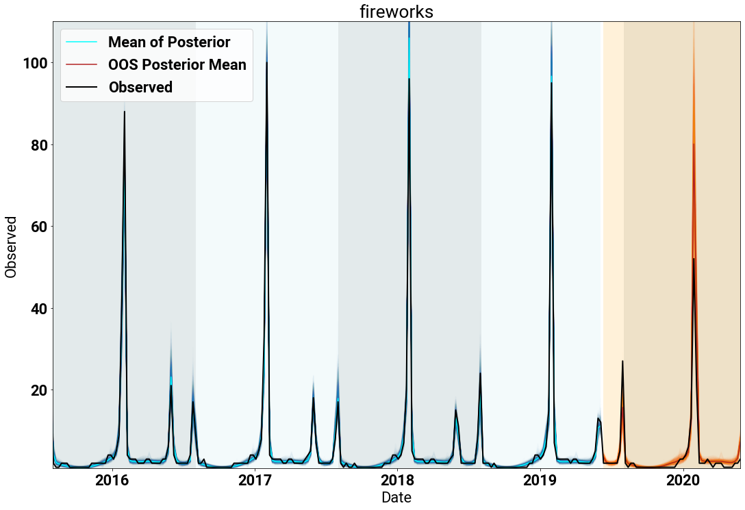
Inspecting the fit, we see the expected spikes for the Fourth of July and New Year’s.
Since our model is additive, we can observe the effect of individual holidays on the observations. The following figure shows the individual posterior traces for each holiday in the last two years of training and the full holdout set.
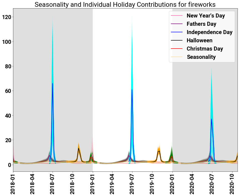
We see that the three spikes in searches are made up of
- A Combinations of New Year’s Day and Christmas
- A Combination of Father’s Day and Independence Day
- Halloween (seemingly)
with a small amount of seasonality to model the fit.
The spikes about Independence Day and New Year’s are expected, but at least for those living in the United States, the activation of Halloween seems very odd! It is not a traditional holiday to expect fireworks. To those living in the Commonwealth, however, there is an obvious explanation: Guy Fawkes Day.
Guy Fawkes day occurs on November 5th. It marks the anniversary of the discovery of a plot to blow up the Houses of Parliament in London in 1605. Within the UK it is customary to have both fireworks and bonfires to celebrate the holiday.
This example shows the importance of having the correct holiday calendar for the data that you are modeling. Having an American calendar to model global data can lead to nonsensical results (as happened in this case). An important caveat is that our model fits the data to a close holiday (Halloween), and this behavior is a good posterior check to see if your calendar is appropriate.
Another interesting insight is the activation of Father’s Day. Father’s Day occurs on the third Sunday of June each year. This is another holiday where we would not expect to see prevalent fireworks. In this instance, by looking at the values of the intensities between Father’s Day and Independence Day, the model attributes searches for fireworks before July 4th both to Independence Day and Father’s Day.
Given the weakly-informative priors for the baseline model, we do not a priori encode any difference between the two holidays, so the model is free to select from either. Knowing we do not expect to see fireworks on Father’s Day, we should update our priors to make it search-term specific (i.e. put a much smaller prior on the intensity for Father’s Day than that of the 4th of July).
The same phenomenon occurs between Christmas and New Year’s: the model estimates the search term counts are due to a split between the two holidays, since no prior information was given to distinguish between them.
Chocolate [11]
The plot below shows a time series of counts for the search term “chocolate” (again in black). Again, the blue lines denote the posterior samples from fitting the model, and the orange lines are the posterior draws for the holdout time period.
The model does a great job of fitting the time series data. In particular, capturing the spikes near Thanksgiving, Christmas and Valentine’s Day. The low-frequency seasonality and baseline capture the remaining counts throughout the year.
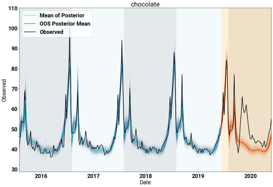
An interesting artifact of the holdout time period, is that the model completely misses the lift in searches around March of 2020. This is due to the model extrapolating from historical data, and there has never historically been a lot of searches for chocolate in March. One thing that also has never occured in March is a large number of people sheltering-in-place due to COVID-19. Perhaps staying at home during a global pandemic makes people want chocolate?
Pumpkin Spice [12]
Our last example shows the power of the model to fit “holidays” that do not fit a typical calendar definition. The search term “Pumpkin Spice” aligns with the (re-)introduction of the Pumpkin Spice Latte (PSL) from Starbucks each autumn.
The fit against the searches below shows a few interesting observations: The first is that the searches occur over a long period of time (early September through late November). The second is that the overall lift is punctuated by spikes of searches in two areas (seemingly early September and mid-November).
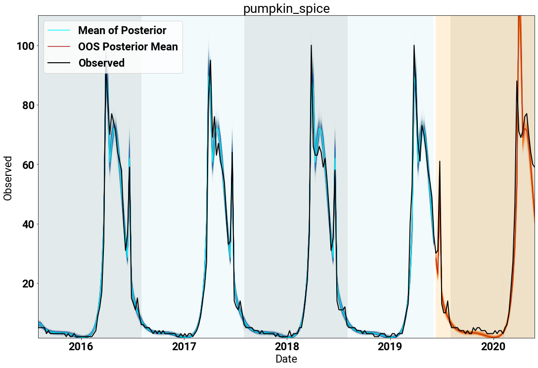
So how is the model fitting this data? Through a combination of seasonality and holiday effects. As seen in the following figure, coupled with the seasonal component modeling the long duration lift, a combination of Labor Day and Thanksgiving lead to the fit we expect for people searching for their PSLs.
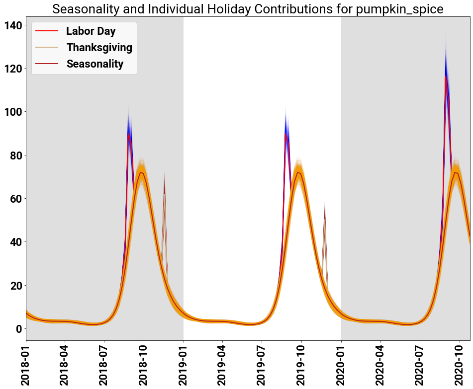
In this example, Labor Day is doing the work of fitting the spike at the beginning of the PSL promotion at Starbucks. Our simplistic model has limited power to capture this dynamic, so it utilizes the closest holiday to the start of the promotion, namely Labor Day. In reality, a Starbuck’s model would probably also include data features like marketing spend and other components that would allow for robust inference in the true domain.
Furthermore, the posterior samples for Labor Day expose a weakness of the model: there is no hard constraint that prevents any holiday from having support for long periods of time. Therefore, Labor Day, which occurs in early September, has support over a full two months leading up to the holiday. An extension of the model would be to enforce compact support for each holiday to be within the time period between the previous to the next holiday. So in this instance, the support for Labor Day could not surpass Independence Day previously, nor exceed Columbus Day/Indiginous People’s Day going forward.
Conclusion
Having a principled holiday effect function embedded within your time series model is crucial to be able to extract knowledge about how holidays affect your observed data.
Being able to decompose individual effects is a powerful tool to determine if your strategies or decisions are doing what you expect. Furthermore, having a flexible model let’s you determine if you are even using the right holiday calendar!
Happy Holidays from all of us at Stitch Fix!!
Attributions
Part of this work was done with Alex Braylan while the author was at Revionics (now Atios), and presented at StanCon Helsinki in August 2018.
References
[2] Tucker S. McElroy, Brian C. Monsell, and Rebecca Hutchinson. “Modeling of Holiday Effects and Seasonality in Daily Time Series.” Center for Statistical Research and Methodology Report Series RRS2018/01. Washington: US Census Bureau (2018).
[3] Usha Ramanathan and Luc Muyldermana. “Identifying demand factors for promotional planning and forecasting: A case of a soft drink company in the UK”. International Journal of Production Economics, 128 (2), 538-545 (2010)
[4] Nari S. Arunraj and Diane Ahrens. “Estimation of non-catastrophic weather impacts for retail industry”. International Journal of Retail and Distribution Management, 44:731–753 (2016)
[5] Florian Ziel. “Modeling public holidays in load forecasting: a German case study”. Journal of Modern Power Systems and Clean Energy 6(2):191–207 (2018).
[6] Sean J. Taylor and Benjamin Letham. “Forecasting at scale”. The American Statistician (2017).
[7] Rob J. Hyndman and George Athanasopoulos. Forecasting: Principles and Practice, online: https://otexts.com/fpp2/ (2012)
[8] Andrew Gelman, Aki Vehtari, Daniel Simpson, Charles C. Margossian, Bob Carpenter, Yuling Yao, Lauren Kennedy, Jonah Gabry, Paul-Christian Bürkner, Martin Modrák. Bayesian Workflow. https://dpsimpson.github.io/pages/talks/Bayesian_Workflow.pdf
[9] Juho Piironen and Aki Vehtari. “Sparsity information and regularization in the horseshoe and other shrinkage priors.” Electronic Journal of Statistics, 11(2): 5018–5051 (2017)
