Although a commonly used phrase, there is no such thing as a “statistically significant sample” – it’s the result that can be statistically significant, not the sample. Word-mincing aside, for any study that requires sampling – e.g. surveys and A/B tests – making sure we have enough data to ensure confidence in results is absolutely critical.
Generally considered to be “stats 101” material, sample size determination is actually a non-trivial task. There is no “optimal” answer that can be derived by fitting a model to a dataset; the answer depends solely on the assumptions and requirements we specify in advance.
The most common way to determine the necessary sample size is through a prospective power analysis – a classic technique that can be used to derive the sample size needed to detect an effect of a given size at a given level of confidence. The purpose of this post is to demystify power analysis for those who are new to data science, as well as to provide some tips that make life easier when determining the necessary sample size. Specifically, we will cover the following areas:
- Overview of hypothesis testing and power analysis for basic A/B testing. If you are an experienced data scientist, you will find this information familiar. If not, this may serve as a useful intro or refresher.
- How to deal with the detectable difference. This is the most important and challenging parameter in power analysis. Specifically, we will discuss how to tie the detectable difference to the business/research context of the study.
- Examples of how to generate power analyses in R using the stats package. We will also demonstrate how to visualize the results with ggplot.
Hypothesis Testing and Power Analysis
In order to understand classic power analysis, you have to understand the basics of frequentist hypothesis testing. Hence we will cover this topic first.
Hypothesis Testing
In order to explain hypothesis testing, we’ll use a classic “intervention” example found in most industries. Let’s say we want to conduct an experiment to test if a certain action helps prevent the occurrence of an adverse event. Depending on the business, this event could be fraud, attrition, downgrades, account closure, etc. The goal is to contact just enough people to decide if the action should be launched at full scale.
Step 1 - Create a null hypothesis and an alternative hypothesis
Defining the null and alternative hypotheses is the first step:
- Null hypothesis (\( H_0 \)): the event rates are the same for the test and control groups
- Alternative hypothesis (\(H_1\)): the event rates are different
Note that the event rate refers to the proportion of clients for whom the event is observed (e.g., fraud, attrition, downgrades, etc.).
The null hypothesis is the hypothesis of no impact, while the alternative hypothesis is that the action will have an impact. This is a two-sided hypothesis, since we are testing if the event rate improved or worsened. An example of a one-sided hypothesis would be to only test if the event rate improved.
Step 2 - Draw a sample
Let’s say we draw a sample of \(N\) clients where 50% are exposed to the action and 50% are not. Note that the split is random, but does not have to be 50/50. We’ll learn how to choose \(N\) later.
Step 3 - Calculate the test statistic
Select the appropriate test statistic and calculate its value from the data (we will call it \(Z\)). A test statistic is a single metric that can be used to evaluate the null hypothesis. For our test the underlying metric is a binary yes/no variable (event), which means that the appropriate test statistic is a test for differences in proportions:
\[Z = \frac{p_1 - {p}_2}{\sqrt{p(1-p) \left(\frac{1}{n_1} + \frac{1}{n_2} \right)}}\]where:
- \( p_1 \) and \( p_2 \) are the event rates for the control and test groups, respectively
- \(n_1\) and \(n_2\) are the sample sizes for the control and test groups, respectively
- \(p\) is the blended rate: \( (x_1+x_2)/(n_1+n_2) \) where \(x_1\) and \( x_2 \) are event counts
Intuitively, this metric makes sense: subtract the rates and normalize the result using the standard error. Moreover, under the null hypothesis (where the expected difference is 0), \(Z\) follows a standard normal distribution with a mean of 0 and standard deviation of 1 if \(N\) is fairly large and \(p\) is not too close to 0 or 1.
For testing of continuous variables, such as revenue, see the appendix of this post.
Step 4 - Reject or accept the null hypothesis
Based on the test statistic we can calculate the p-value which is probability of obtaining a result at least as “extreme” as the observed result, given that the null hypothesis is true. It is tempting to interpret the p-value as the probability of rejecting the null hypothesis when it is true, but technically speaking that is an incorrect interpretation. The p-value is based on frequentist inference, as opposed to Bayesian inference, and hence does not provide any measure of probability about the hypothesis. For more on this, see my Bayesian post (link provided below).
If we seek to reject the null hypothesis, we want the p-value to be small and the typical threshold used is \(5\%\). In other words, if the p-value is less than \(5\%\), and the test group experienced a lower event rate than the control group, we conclude that the action worked. The pre-chosen cutoff (\(5\%\)) is also referred to as the significance level and plays an important role in determining the required sample size. We will explain the significance level in the following section.
Note that we do not have to calculate the p-value in order to reject or accept the null hypothesis. Alternatively, we can apply a cutoff directly to the test statistic based on its distribution and the chosen significance level. For example, for a two-sided test and a significance level of \(5\%\), the cutoff corresponds to the upper and lower \(2.5\%\) on the standard normal distribution (normal distribution with a mean of 0 and a standard deviation of 1), which is \(1.96\). Hence we reject the null hypothesis if \(|Z|>1.96\).
Introducing the Power and the Significance Level
In the world of hypothesis testing, rejecting the null hypothesis when it is actually true is called a type 1 error. Committing a type 1 error is a false positive because we end up recommending something that does not work.
Conversely, a type 2 error occurs when you accept the null hypothesis when it is actually false. This is a false negative because we end up sitting on our hands when we should have taken action. We need to consider both of these types of errors when choosing the sample size.
| \(H_0\) is true | \(H_1\) is true | |
| Accept \(H_0\) | Correct Decision | Type 2 Error (1 - power) |
| Reject \(H_0\) | Type 1 Error (significance level) | Correct decision |
Two important probabilities related to type 1 and type 2 error:
- The probability of committing a type 1 error is called the significance level.
- The probability of committing a type 2 error is called the power.
A typical requirement for the power is \(80\%\). In other words, we will tolerate a \(20%\) chance of a type 2 error (1 - power). As mentioned above, the typical requirement for the significance level is \(5\%\).
Visual Representation of the Power and the Significance Level
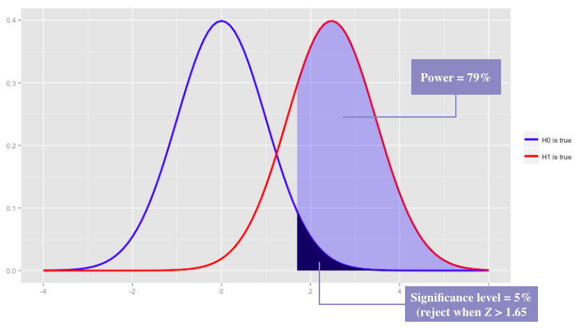
The concepts of power and significance level can seem somewhat convoluted at first glance. A good way to get a feel for the underlying mechanics is to plot the probability distribution of \(Z\) assuming that the null hypothesis is true. Then do the same assuming that the alternative hypothesis is true, and overlay the two plots.
Consider the following example:
- \(H_0\): \(p_1=p_2\), \(H_1\): \(p_1>p_2\). A one-sided test was chosen here for charting-simplicity.
- Our chosen significance level is \(5\%\). The corresponding decision rule is \(|Z| > 1.65\). The number (\(1.65\)) is the cutoff that corresponds to the upper \(5\%\) on the standard normal distribution.
- \(N = 5,000\) (\(2,500\) in each cell).
- Say we decide that we need to observe a difference of \(0.02\) in order to be satisfied that the intervention worked (i.e., \(p_1 = 0.10\) and \(p_2 = 0.08\)). We will discuss how to make this decision later in the post. The desired difference of \(0.02\) under the alternative hypothesis corresponds to \(Z=2.47\) (using the formula for \(Z\) above). We are assuming that the variance is roughly the same under the null and alternative hypotheses (they’re very close).
R Code
x <- seq(-4, 6, 0.1)
mean1 <- 0.00
mean2 <- 2.47
dat <- data.frame(x = x, y1 = dnorm(x, mean1, 1), y2 = dnorm(x, mean2, 1))
ggplot(dat, aes(x = x)) +
  geom_line(aes(y = y1, colour = 'H0 is true'), size = 1.2) +
  geom_line(aes(y = y2, colour = 'H1 is true'), size = 1.2) +
  geom_area(aes(y = y1, x = ifelse(x > 1.65, x, NA)), fill = 'black') +
  geom_area(aes(y = y2, x = ifelse(x > 1.65, x, NA)), fill = 'blue', alpha = 0.3) +
  xlab("") + ylab("") + theme(legend.title = element_blank()) +
  scale_colour_manual(breaks = c("H0 is true", "H1 is true"), values = c("blue", "red"))
Graph Produced by the R Code
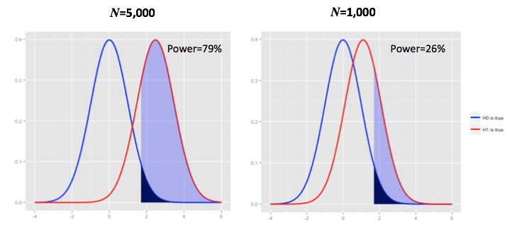
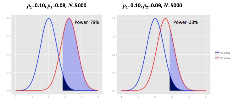
Note that if we pick a smaller \(N\), or a smaller difference between \(p_2\) and \(p_1\), the power drops:
Power Analysis
Let’s say we require the significance level to be 5% and the power to be \(80\%\). This means we have now specified two key components of a power analysis:
- A decision rule of when to reject the null hypothesis. We reject the null when the p-value is less than \(5\%\).
- Our tolerance for committing type 2 error (\(1 - 80\% = 20\%\)).
Our next task now is to find the sample size that meets these two criteria. On the surface this sounds easy, but it actually poses a challenge. In fact, this is akin to solving one equation (\(\textrm{power}=80\%\)) with two unknowns: the sample size and the detectable difference. The detectable difference is the level of impact we want to be able to detect with our test. It is almost always the bottleneck in a power analysis and directly dictates the precision of the sample. We cannot solve for the sample size without first specifying the level of impact we want to be able to detect with our test.
In order to explain the dynamics behind this, let’s go back to the definition of power: the power is the probability of rejecting the null hypothesis when it is false. Hence for us to calculate the power, we need to define what “false” means to us in the context of the study. In other words, how much impact, i.e., difference between test and control, do we need to observe in order to reject the null hypothesis and conclude that the action worked?
Let’s consider two illustrative examples: if we think that an event rate reduction of, say, \(10^{-10}\) is enough to reject the null hypothesis, then we need a very large sample size to get a power of \(80\%\). This is pretty easy to deduce from the charts above: if the difference in event rates between test and control is a small number like \(10^{-10}\), the null and alternative probability distributions will be nearly indistinguishable. Hence we will need to increase the sample size in order to move the alternative distribution to the right and gain power. Conversely, if we only require a reduction of \(0.02\) in order to claim success, we can make do with a much smaller sample size. The smaller the detectable difference, the larger the required sample size.
The next section provides some mathematical details behind this. After that, we’ll discuss how to choose the detectable difference.
Power Analysis – Some Mathematical Details
We will return to the two-sided test example for this section since it is more general. For a two-sided test, at a significance level of \(5\%\), we will reject the null hypothesis when \(|Z| > 1.96\) (the number \(1.96\) is the cutoff that corresponds to \(2.5\%\) on the standard normal distribution). Based on this decision rule, we can then find an N such that the power equals \(80\%\). This can be solved by adding the lower-sided and upper-sided powers:
\[P(Z < A) + P(Z > B) = 0.80\]where \(A\) and \(B\) are defined as:
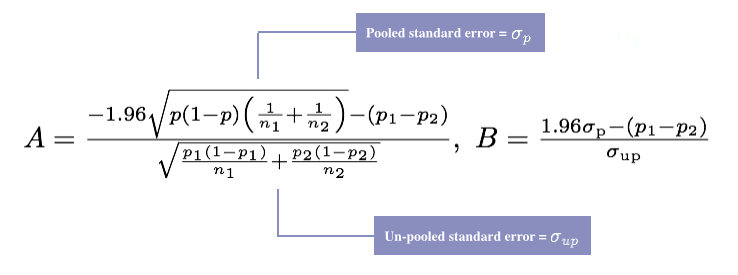
Note that \(A\) and \(B\) are merely variables used to simplify the expression.
Clearly, as mentioned in the section above, the power equation above does not just depend on \(N\), it also depends on \(p_1\) and \(p_2\). Hence we need to specify the detectable difference (\(p_1 – p_2\)) in order to solve for \(N\).
Choosing the Detectable Difference
Unlike the significance level and the power, there are no plug-and-play values we can use for the detectable difference. However, if we put the detectable difference in the context of what we are trying to get out of the study, things become more clear. First, let’s start with some guiding principles and then move on to specific suggestions:
Avoid wasteful sampling: Let’s say it takes an absolute difference of \(0.02\) between test and control in order for the treatment to pay off. In this case, aiming for a 0.01 detectable difference would just lead to more precision than we really need. Why have the ability to detect 0.01 if we don’t really care about a \(0.01\) difference? If there is no cost to sampling and/or you have an infinite pool of clients to choose from, this is a moot point. But in many cases, sampling for unnecessary precision can be costly, financially or in terms of over-contacting your clients.
Avoid missed opportunities: Conversely, if we are analyzing a sensitive metric where small changes can have a large impact, we have to aim for a small detectable difference. If we choose an insufficient sample size, we may end up sitting on our hands and missing an opportunity (type 2 error).
Clearly, the key is to define what “pay off” means for the study at hand, which depends on what the adverse event is a well as the cost of the action. Hence the answer should come from a cross-functional analysis/discussion between the data scientist and the business stakeholder.
Starting a Productive Discussion About the Detectable Difference
Start the discussion by providing viable suggestions that people can react to. Below are a couple of ways to think about the problem that all adhere to the guiding principles (in the context of an A/B test). We will break into two separate use cases based on whether or not there is a financial cost associated with the treatment. When there is a cost involved, the detectable difference can be pegged to the break-even point of the tactic. If the treatment is “free” the detectable difference can be pegged to the minimal overall impact that would make the test worth the time and effort.
Break-even Analysis
If there is a non-trivial marginal cost associated with the treatment, we don’t need the ability to detect small differences that will lead to a negative ROI. In other words, we wouldn’t take action if the null hypothesis is rejected and hence a large and powerful sample may be a waste. In summary, find the the detectable difference that corresponds to the break-even point of the tactic.
Overall Impact Analysis
The ROI-based approach outlined above can lead to an unreasonably small detectable difference (and thus overly large samples) when the marginal cost is low or non-existent (e.g., email campaigns). In this case, the best approach is to estimate the impact from deploying the program at full scale at different levels of impact. Then, choose the detectable difference that corresponds to the smallest meaningful change. Clearly, this is fuzzy and hence illustrates the importance of having a cross-functional discussion.
Running Power Analyses in R
Once we have a viable range for the detectable difference, we can evaluate the sample size required for each option. This is easy to do in R using the code below. Here we are using the basic power functionalities in core R, but if you are running more complex analyses the pwr package may come in handy.
For example, let’s say that \(p_1 = 0.10\) and we want the detectable difference to be between \(0.01\) and \(0.03\). Clearly, we’d rather be able to detect a difference of \(0.01\) but it may be too costly and hence we want to evaluate more conservative options as well.
library(scales)
library(ggplot2)
p1 <- 0.1 # baseline rate
b <- 0.8 # power
a <- 0.05 # significance level
dd <- seq(from = 0.01, to = 0.03, by = 0.0001) # detectable differences
result <- data.frame(matrix(nrow = length(dd), ncol = 2))
names(result) <- c("DD", "ni")
for (i in 1:length(dd)) {
  result[i, "DD"] <- dd[i]
  result[i, "ni"] <- power.prop.test(sig.level = a, p1 = p1, p2 = p1 - dd[i],
                                     alternative = 'two.sided', power = b)\\(n
}
ggplot(data = result, aes(x = DD, y = ni)) +
  geom_line() + ylab("n") + xlab("Detectable difference") + scale_x_continuous(labels = comma) +
  geom_point(data = result[ceiling(result\\(n / 10) * 10 == 5000, ],
             aes(x = DD, y = ni), colour = "red", size = 5)
Sample Size Requirements at Different Levels of Detectable Difference
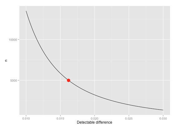
(Note that the \(n\) here is the sample size needed for each cell - i.e., \(n = n_1 = n_2\) and \(n_1 + n_2 = N\).)
This graph shows that we need roughly 10x more observations to get a detectable difference of \(0.01\) compared to \(0.03\). This is because the power increases with \( \sqrt{N} \). Hence, settling for a detectable difference around the middle of the range in terms of sample size requirement – e.g., \(0.016\) – is perhaps the most prudent choice. This leads to a decent power at a sample size of \(10,000\) (\(5,000\) in each cell). Again, this is a made-up example and you can easily plug your own numbers into the code:
power.prop.test(sig.level=0.05, p1=0.1, p2=0.10-0.016, alternative='two.sided', n=5000)$power
[1] 0.7905305
Final Remarks
Power analysis is challenging because it depends completely on assumptions and requirements we specify in advance. While we can comfortably rely on industry standard requirements for the power and the significance level, there are no such options for the detectable difference. However, if we follow some basic guiding principles, we should be able to find a detectable difference that satisfied all constituents. Specifically, the chosen detectable difference should incorporate the business context of the tactic that is being tested – e.g., ROI, and should be discussed in a cross-functional setting.
We should note that the use case covered in this post is a simple A/B test with equal sample sizes for test and control groups. Obviously, experimental designs and sampling schemes can get more much complex, but the underlying philosophy and approach are the same. And in all cases you will benefit from considering the business context when choosing the detectable difference.
Last but not least, Bayesian approaches to sample size determination exist as well. However, depending on your level of comfort with random distributions and Monte Carlo techniques, it may also be more challenging to execute. For more on Bayesian versus frequentist statistics, see this post on the Stitch Fix technology blog.
Appendix: Power Analysis for Continuous Variables
In the example above, we did a test of proportions since the underlying outcome variable is binary. When comparing averages of continuous variables across two samples (such as revenue), the simplest test statistic is the t-test. This test statistic is similar to the test we use for proportions – i.e., subtract the means and divide by the pooled standard error. However, the detectable differences are typically expressed in terms of the effect size given by:
\[D = \frac{\bar{X}_1 - \bar{X}_2}{S}\]where \(S\) is the pooled standard deviation, \(X_1\) is the average of the control group, and \(X_2\) is the average of the test group. When choosing the \(D\), we can follow the suggested framework above for the detectable difference. Another option is to use Cohen’s guidelines for small, medium, and large effects (\(D = 0.2, 0.5, 0.8\)). However, these values are tied to the historical variance of the data (the \(S\) in the denominator) as opposed to the business context.
In order to run these types of tests in R, simply replace power.prop.test with power.t.test.
R Code
library(ggplot2)
es <- seq(from = 0.1, to = 0.3, by = 0.001) # effect sizes
result <- data.frame(matrix(nrow = length(es), ncol = 2))
names(result) <- c("ES", "ni")
for (i in 1:length(es)){
  result[i, "ES"] <- es[i]
  result[i, "ni"] <- power.t.test(sig.level = a, d = es[i], sd = 1,
                                  alternative = 'two.sided', power = b)$n
}
ggplot(data = result, aes(x = ES, y = ni)) + geom_line() + xlab("Effect Size") + ylab("N") +
  scale_x_continuous(labels = comma)