Binary classification models are perhaps the most common use-case in predictive analytics. The reason is that many key client actions across a wide range of industries are binary in nature, such as defaulting on a loan, clicking on an ad, or terminating a subscription.
Prior to building a binary classification model, a common step is to perform variable screening and exploratory data analysis. This is the step where we get to know the data and weed out variables that are either ill-conditioned or simply contain no information that will help us predict the action of interest. Note that the purpose of this step should not to be confused with that of multiple-variable selection techniques, such as stepwise regression and lasso, where the variables that go into the final model are selected. Rather, this is a precursory step designed to ensure that the approaches deployed during the final modeling phases are set up for success.
The weight of evidence (WOE) and information value (IV) provide a great framework for for exploratory analysis and variable screening for binary classifiers. WOE and IV have been used extensively in the credit risk world for several decades, and the underlying theory dates back to the 1950s. However, it is still not widely used outside the credit risk world and it is a somewhat underserved area in R.
WOE and IV enable one to:
- Consider each variable’s independent contribution to the outcome.
- Detect linear and non-linear relationships.
- Rank variables in terms of “univariate” predictive strength.
- Visualize the correlations between the predictive variables and the binary outcome.
- Seamlessly compare the strength of continuous and categorical variables without creating dummy variables.
- Seamlessly handle missing values without imputation.
- Assess the predictive power of missing values.
In this paper we will provide a brief description of WOE and IV as well as the Information R package, which provides an easy way to perform variable screening and exploratory analysis with WOE and IV for traditional binary classifiers as well as uplift models.
What Are WOE and IV?
Background
Weight of evidence (WOE) and information value are closely related to concepts from information theory where one of the goals is to understand the uncertainty involved in predicting the outcome of random events given varying degrees of knowledge of other variables (see [2], [3], and [4]). Thus this is a perfect framework for variable screening and exploratory analysis for predictive modeling.
Information theory kicked off when Claude Shannon (1948) wrote down an expression for the entropy of a probability distribution. Entropy is often described as the level of “disorder,” but in the context of information theory it is better to think of it as one’s level of uncertainty. High entropy means high uncertainty (you don’t know what tomorrow holds) and low entropy mean low uncertainty (there will be no surprises tomorrow).
Suppose a friend tosses a coin and asks you to predict whether the toss came up heads or tails. There’s 50 percent probability of each possibility, so your prediction isn’t worth very much. This turns out to be the maximum amount of entropy for an event with two possible outcomes. Suppose instead that you know the coin is weighted so that it comes up heads 90 percent of the time. Now your job of making a prediction is easier – Shannon’s formula tells you exactly how much information you’ve gained compared to the previous situation.
Mutual information is a way of summarizing much knowing the value of one random variable tells you about another random variable (Shannon + Weaver 1949). If \(X\) and \(Y\) are independent, the mutual information is zero. Any correlations (positive, negative, or nonlinear) will result in positive mutual information. It turns out the mutual information of \(X\) and \(Y\) is nicely expressed in terms of entropy (\(H\)):
\[\text{MI}(X,Y) = H(X) + H(Y) - H(X,Y). \nonumber\]Mutual information is the difference in predictability that you get from knowing the joint distribution \(p(X,Y)\) compared to knowing only the two marginal distributions \(p(X)\) and \(p(Y)\).
Information value (IV), which we will define below, is quite closely connected to mutual information (MI), and both are intended to do the same thing: summarize how much knowing the value of \(X\) in a given trial helps you predict the value of \(Y\) for the same trial.
Setup
Let’s say that we have a binary dependent variable \(Y\) and a set of predictive variables \(X_1, \ldots, X_p\). As mentioned above, \(Y\) can capture a wide range of outcomes, such as defaulting on a loan, clicking on an ad, or terminating a subscription.
WOE and IV play two distinct roles when analyzing data:
- WOE describes the relationship between a predictive variable and a binary target variable.
- IV measures the strength of that relationship.
The Weight of Evidence
The WOE/IV framework is based on the following relationship:
\[\log \frac{P(Y=1 | X_j)}{P(Y=0 | X_j)} = \underbrace{\log \frac{P(Y=1)}{P(Y=0)}}_{\text{sample log-odds}} + \underbrace{\log \frac{f(X_j | Y=1)}{f(X_j | Y=0)}}_{\text{WOE}}, \nonumber\]where \(f ( x_j \| Y )\) denotes the conditional probability density function (or a discrete probability distribution if \(X_j\) is categorical).
This relationship says that the conditional logit of \(P(Y=1\), given \(X_j\), can be written as the overall log-odds (i.e., the “intercept”) plus the log-density ratio – also known as the weight of evidence.
Note that the weight of evidence and the conditional log odds of \(Y=1\) are perfectly correlated since the “intercept” is constant. Hence, the greater the value of WOE, the higher the chance of observing \(Y=1\). In fact, when WOE is positive the chance of of observing \(Y=1\) is above average (for the sample), and vice versa when WOE is negative. When WOE equals 0 the odds are simply equal to the sample average.
Ties to Naive Bayes and Logistic Regression
Notice that the left-hand-side of the equation above – i.e., the conditional log odds – is exactly what we are trying to predict in a logistic regression model. Hence, when building a logistic regression model – which is perhaps the most widely used technique for building binary classifiers – we are actually trying to estimate the weight of evidence.
Last, but not least, the WOE framework has ties to the well-known naive Bayes classifier, given by (see [1]):
\[\log \frac{P(Y=1| x_1, \ldots, x_p)}{P(Y=0 | x_1, \ldots, x_p)} = \log \frac{P(Y=1)}{P(Y=0)} + \sum_{j=1}^p \log \frac{f(X_j | Y=1)}{f(X_j | Y=0)}. \nonumber.\]The naive Bayes model essentially says that the conditional log odds is equal to the sum of the individual weight of evidence vectors. The word “naive” comes from the fact that this model relies on the assumption that all predictors are conditionally independent given \(Y\), which is a highly optimistic assumption.
In the credit scoring industry a “semi-Naive” version of this model is quite popular. The idea is to transform the data into WOE vectors and then use logistic regression to fit the model
\[\log \frac{P(Y=1| x_1, \ldots, x_p)}{P(Y=0 | x_1, \ldots, x_p)} = \log \frac{P(Y=1)}{P(Y=0)} + \sum_{j=1}^p \beta_j \log \frac{f(X_j | Y=1)}{f(X_j | Y=0)}, \nonumber\]thus partly relaxing the assumption that all predictors in the model are independent. It should be noted that the underlying WOE vectors are still estimated univariately and that the coefficients merely function as scalars. For a more general model, GAM is a great choice (see [5]).
Measuring Univariate Variable Strength with the Information Value
We can leverage WOE to measure the predictive strength of \(x_j\) – i.e., how well it helps us separate cases when \(Y=1\) from cases when \(Y=0\). This is done through the information value (IV) which is defined like this:
\[\text{IV}_j = \int \log \frac{f(X_j | Y=1)}{f(X_j | Y=0)} \, (f(X_j | Y=1) - f(X_j | Y=0)) \, dx. \nonumber\]Note that the IV is essentially a weighted “sum” of all the individual WOE values where the weights incorporate the absolute difference between the numerator and the denominator (WOE captures the relative difference). Generally, if \(\text{IV} < 0.05\) the variable has very little predictive power and will not add any meaningful predictive power to your model.
Estimating WOE
The most common approach to estimating the conditional densities needed to calculate WOE is to bin \(X_j\) and then use a histogram-type estimate.
Here is how it works: create a \(k \times 2\) table where \(k\) is the number of bins, and the cells within the two columns count the number of records where \(Y=1\) and \(Y=0\), respectively. The bins are typically selected such that the bins are roughly evenly sized with respect to the number of records in each bin (if possible). The conditional densities are then obtained by calculating the “column percentages” from this table. The typical number of bins used is 10-20. If \(X_j\) is categorical, no binning is needed and the histogram estimator can be used directly. Moreover, missing values are treated as a separate bin and thus handled seamlessly.
If \(B_1, \ldots, B_k\) denote the bins for \(X_j\), the WOE for \(X_j\) for bin \(i\) can be written as
\[\text{WOE}_{ij} = \log \frac{P(X_j \in B_i | Y=1)}{P(X_j \in B_i | Y=0)}, \nonumber\]which means that the IV for variable \(X_j\) can be calculated as
\[\text{IV}_j = \sum_{i=1}^k (P(X_j \in B_i | Y=1) - P(X_j \in B_i | Y=0)) \times \text{WOE}_{ij}. \nonumber\]Extensions to Exploratory Analysis for Uplift Models
Consider a direct marketing program where a test group received an offer of some sort and the control group did not receive anything. The test and control groups are based on a random split. The lift of the campaign is defined as the difference in success rates between the test and control groups. In other words, the program can only be deemed successful if the offer outperforms the “do nothing” (a.k.a baseline) scenario.
The purpose of uplift models is to estimate the difference between the test and control groups and then using the resulting model to target persuadables – i.e., potential or existing clients that are on the fence and need some sort of offer to buy a product. Thus, when preparing to build an uplift model, we cannot only focus on the log odds of \(Y=1\), we also need to consider the log odds ratio of \(Y=1\) for the test group versus the control group. This leads to the net weight of evidence (NWOE) and the net information value (NIV). (Actual uplift modeling techniques are beyond the scope of this paper; we will stick to model exploration and variable screening.)
The net weight of evidence (NWOE) is the difference between the WOEs for the test group (\(\text{WOE}_{t}\)) and the control group (\(\text{WOE}_{c}\)),
\[\text{NWOE} = \text{WOE}_{t} - \text{WOE}_{c}, \nonumber\]which is equivalent to
\[\text{NWOE}_j = \log \frac{f(x_j|Y=1)_{t}f(x_j|Y=0)_{c}}{f(x_j|Y=1)_{c}f(x_j|Y=0)_{t}}. \nonumber\]The net information value for variable \(X_j\) is then defined as
\[\int \left( f(X_j|Y=1)_{t}f(X_j|Y=0)_{c} - f(X_j|Y=1)_{c}f(X_j|Y=0)_{t} \right) \times \log \frac{f(X_j|Y=1)_{t}f(X_j|Y=0)_{c}}{f(X_j|Y=1)_{c}f(X_j|Y=0)_{t}} \, dx_j.\]NWOE and NIV work just like IV and WOE, just from an uplift perspective. NIV measures the strength of a given variable while NWOE describes the pattern of the relationship. Specifically, the higher the value of NIV, the better the given variable is at separating self-selectors – i.e., people who are self-motivated to buy – and persuadables that need to be motivated.
The Information R Package
The information package is designed to perform exploratory data analysis and variable screening for binary classification models using WOE and IV. To make the package as efficient as possible aggregations are done in data.table and creation of WOE vectors can be distributed across multiple cores.
The package can be downloaded from https://github.com/klarsen1/Information.
There are a number of R packages available that support WOE and IV (see a partial list below), but they are either primarily designed to build WOE-based models – e.g., naive Bayes classifiers – or they do not support the uplift use-case.
Date Used in Examples
The data is from an historical marketing campaign from the insurance industry and is automatically downloaded when you install the Information package. The data is stored in two .RDA files, one for the training dataset and one for the validation dataset. Each file has 68 predictive variables and 10k records.
The datasets contain two key indicators:
PURCHASEThis variable equals 1 if the client accepted the offer, and 0 otherwiseTREATMENTThis variable equals 1 if the client was in the test group (received the offer), and 0 otherwise.
Key Functions
CreateTables()creates WOE tables and IVs for all variables in the input dataframe.PlotWOE()plots the WOE vector for one variable.MultiPlotWOE()plots more than one WOE vector on one page for comparisons.
The same functions work for NWOE and NIV.
The examples below show how to call these functions
External Cross Validation
The information package supports external cross validation to check that the WOE and NWOE vectors are stable.
Let’s assume that we have a training and a validation dataset, and we calculate WOE for both datasets using the same bin cutoffs. The cross validation penalty for bin \(B_i\) is given by
\[\text{penalty}_i = | \text{WOE}_{\text{train}} - \text{WOE}_{\text{valid}} | \nonumber,\]and the total cross validation (CV) penalty is
\[\sum_{i=1}^k |P(X_j \in B_i | Y=1) - P(X_j \in B_i | Y=0)| \times \text{penalty}_i \nonumber.\]where the probabilities used to form the weights are from the training data. The adjusted IV is then defined as
\[\text{NIV} = \text{IV} - \text{total CV penalty} .\nonumber\]The same approach can be applied to NIV for the uplift use-case.
Example for a Traditional Binary Classification Problem
Ranking All Variables Using Adjusted IV
library(Information)
library(gridExtra)
options(scipen=10)
### Loading the data
data(train, package="Information")
data(valid, package="Information")
### Exclude the control group
train <- subset(train, TREATMENT==1)
valid <- subset(valid, TREATMENT==1)
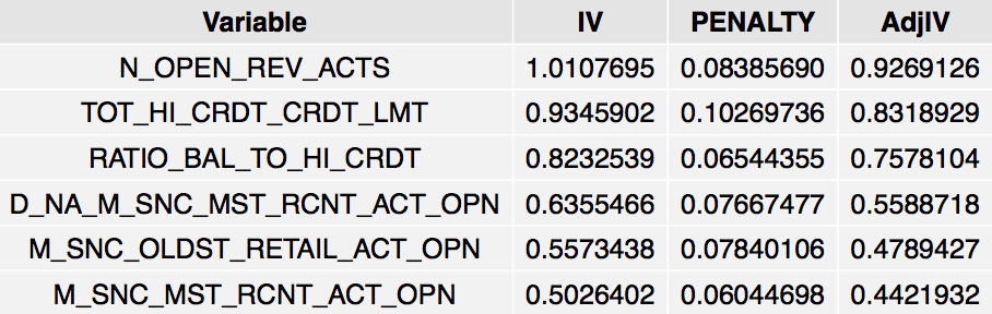
### Ranking variables using penalized IV
IV <- CreateTables(data=train,
valid=valid,
y="PURCHASE")
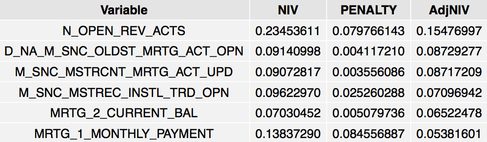
grid.table(head(IV$Summary), rows=NULL)
The strongest six variables:
Analyzing WOE Patterns
The IV$Tables object returned by Information is simply a list of dataframes that contains the WOE tables for all variables in the input dataset. Note that the penalty and IV columns are cumulative.
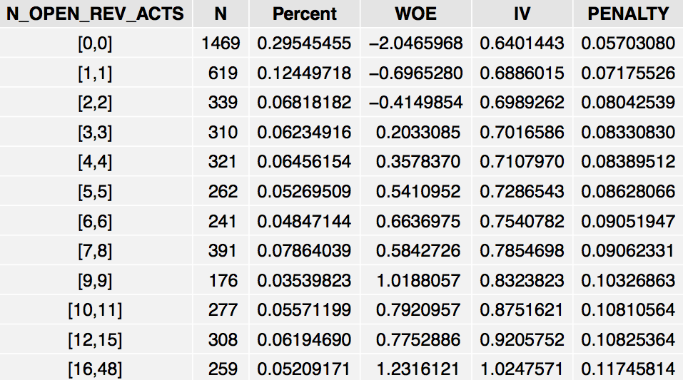
grid.table(IV$Tables$N_OPEN_REV_ACTS, rows=NULL)
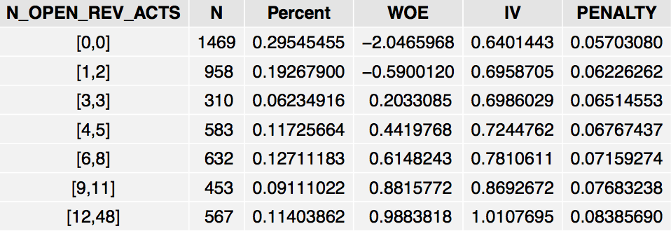
The table shows that the odds of PURCHASE=1 increases as N_OPEN_REV_ACTS increases, although the relationship is not linear.
Note that the Information package attempts to create evenly-sized bins in terms of the number of subjects in each group. However, this is not always possible due to ties in the data, as with N_OPEN_REV_ACTS which has ties at 0. If the variable under consideration is categorical, its distinct categories will show up as rows in the WOE table. Moreover, if the variable has missing values, the WOE table will contain a separate “NA” row which can be used to gauge the impact of missing values. Thus, the framework seamlessly handles missing values and categorical variables without any dummy-coding or imputation .
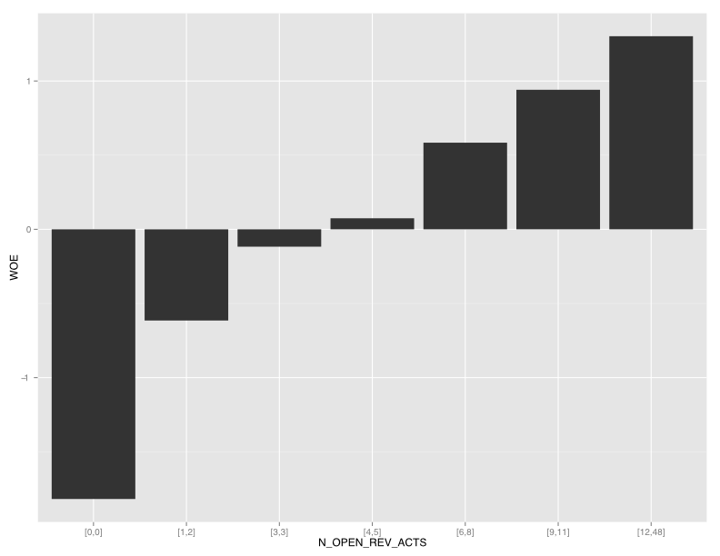
Plotting WOE Patterns
We can also plot this pattern for better visualization:
PlotWOE(IV, "N_OPEN_REV_ACTS")
If we want to plot all variables on separate pages, we can loop through all variables:
n <- names(IV$Tables)
for (i in 1:length(n)){
   PlotWOE(IV, n[i])
}
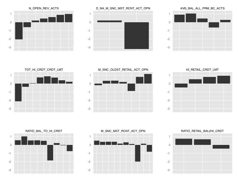
For better visualization we can do a multiplot to compare WOE patterns. Here we plot the first nine variables on one page. Note that we can plot as many variables as we want; MultiPlotWOE will simply spread the plots over multiple pages (max of nine plots per page).
MultiPlotWOE(IV, IV$Summary$Variable[1:9])
Omitting Cross Validation
To run IVs without external cross validation, simply omit the validation dataset:
IV <- CreateTables(data=train, y="PURCHASE")
Changing the Number of Bins
The default number of bins is 10 but we can choose a different number if we desire more granularity. Note that the IV formula is fairly invariant to the number of bins. Also, note that the bins are selected such that the bins are evenly sized, to the extent that it is possible (depending on the number of ties in the data).
IV <- CreateTables(data=train,
                   valid=valid,
                   y="PURCHASE",
                   bins=20)

grid.table(IV$Tables$N_OPEN_REV_ACTS,
           gp=gpar(fontsize=12),
           rows=NULL)
Uplift Example
For an uplift model we have to include both the test group and the control group in our dataset:
data(train, package="Information")
data(valid, package="Information")
When calling the CreateTables function, all we have to do is specify the variable that identifies the test and control groups.
NIV <- CreateTables(data=train,
valid=valid,
y="PURCHASE",
trt="TREATMENT")
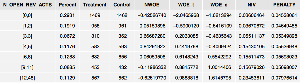
grid.table(head(NIV$Summary),
rows=NULL,
gp=gpar(fontsize=12))
Note that we cannot compare the scales of NIV and IV. Moreover, there is no rule-of-thumb cutoff for the NIV. Hence, we have to use it solely as a ranking statistic and make a judgement call.
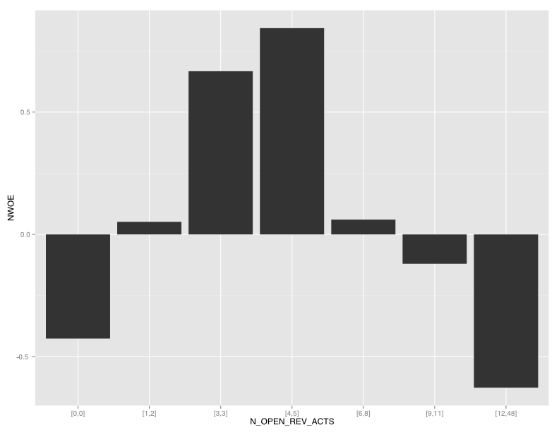
Interestingly, N_OPEN_REV_ACTS is also the most predictive variable from an uplift perspective. However, the NWOE pattern is quite different from the WOE pattern and suggests a u-shaped pattern. This illustrates how the story can be very different when modeling the incremental effect as opposed to simply building a model to estimate the chance of \(Y=1\) following a treatment.
Combining IV Analysis With Variable Clustering
Variable clustering divides a set of numeric variables into mutually exclusive clusters. The algorithm attempts to generate clusters such that
- the correlations between variables assigned to the same cluster are maximized.
- the correlations between variables in different clusters are minimized.
Using this algorithm we can replace a large set of variables by a single member of each cluster, often with little loss of information. The question is which member to choose from a given cluster. One option is to choose the variable that has the highest multiple correlation with the variables within its cluster, and the lowest correlation with variables outside the cluster. A more meaningful choice for a predictive modeling is to choose the variable that has the highest information value. The following code shows how to do this.
In R, we can do this with the ClustOfVar package.
library(ClustOfVar)
library(reshape2)
library(plyr)

data(train, package="Information")
data(valid, package="Information")
train <- subset(train, TREATMENT==1)
valid <- subset(valid, TREATMENT==1)

tree <- hclustvar(train[,!(names(train) %in% c("PURCHASE", "TREATMENT"))])
nvars <- length(tree[tree$height<0.7])
part_init<-cutreevar(tree,nvars)$cluster
kmeans<-kmeansvar(X.quanti=train[,!(names(train) %in% c("PURCHASE", "TREATMENT"))],init=part_init)
clusters <- cbind.data.frame(melt(kmeans$cluster), row.names(melt(kmeans$cluster)))
names(clusters) <- c("Cluster", "Variable")
clusters <- join(clusters, IV$Summary, by="Variable", type="left")
clusters <- clusters[order(clusters$Cluster),]
clusters$Rank <- ave(-clusters$AdjIV, clusters$Cluster, FUN=rank)
selected_members <- subset(clusters, Rank==1)
selected_members$Rank <- NULL
Using variable clustering in combination with IV cuts the number of variables from 68 to 21:
nrow(selected_members)
> 21
nrow(clusters)
> 69
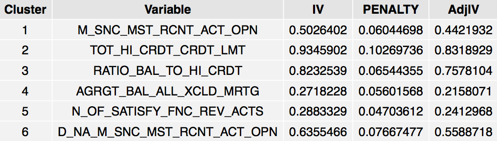
Here are the first rows from the resulting variable ranking table:
grid.table(head(selected_members),
           rows=NULL,
           gp=gpar(fontsize=12))
Summary
-
The purpose of exploratory analysis and variable screening is to get to know the data and assess “univariate” predictive strength, before we deploy more sophisticated variable selection approaches.
-
The weight of evidence (WOE) and information value (IV) provide a great framework for performing exploratory analysis and variable screening prior to building a binary classifier (e.g., logistic regression). It seamlessly handles missing values and character variables, and the output is easy to interpret.
-
The information value originates from information theory and is closely related to the concept of mutual information (see [3], [4]).
-
The information package is specifically written to perform this type of analysis using parallel processing. It also supports exploratory analysis for uplift models, a growing area within marketing analytics. The information package is not designed to transfer data into WOE vectors for Naive Bayes models, although this feature could be added later.
References
[1] Hastie, Trevor , Tibshirani, Robert and Friedman, Jerome. (1986), Elements of Statistical Learning, Second Edition, Springer, 2009.
[2] Kullback S., Information Theory and Statistics, John Wiley & Sons, 1959.
[3] Shannon, C.E., “A Mathematical Theory of Communication”, Bell System Technical Journal, 1948.
[4] Shannon, CE. and Weaver, W. The Mathematical Theory of Communication. Univ of Illinois Press, 1949.
[5] GAM: the Predictive Modeling Silver Bullet, http://multithreaded.stitchfix.com/blog/2015/07/30/gam/.
Other Packages that support WOE/IV
woe package,https://cran.r-project.org/web/packages/woe/woe.pdf.
riv package (not to be confused with the riv packake in CRAN), http://www.r-bloggers.com/r-credit-scoring-woe-information-value-in-woe-package/.
klaR package, https://cran.r-project.org/web/packages/klaR/klaR.pdf.