Introduction
If you ever spent time in the field of marketing analytics, chances are that you have analyzed the existence of a causal impact from a new local TV campaign, a major PR event, or the emergence of a new local competitor. From an analytical standpoint these types of events all have one thing in common: The impact cannot be tracked at the individual customer level and hence we have to analyze the impact from a bird’s eye view using time series analysis at the market level. Data science may be changing at a fast pace but this is an old-school use-case that is still very relevant no matter what industry you’re in.
Intervention analyses typically require more judgement than evaluation of randomized test/control studies. Specifically, when analyzing interventions through time series analysis we typically go through two steps, each of which can involve multiple analytical decisions:
- Finding matching control markets for the test market where the event took place using time series matching based on historical data prior to the event (the “pre period”).
- Analyzing the causal impact of the event by comparing the observed data for the test and control markets following the event (the “post period”), while factoring in differences between the markets prior to the event.
The purpose of this document is to describe a robust approach to intervention analysis based on two key R packages: the CausalImpact package written by Kay Brodersen at Google and the dtw package available in CRAN. In addition, we will introduce an R package called MarketMatching which implements a simple workflow based on these two packages. Last, but not least, the document provides some technical details on two key techniques needed to do intervention analysis: dynamic time warping and Bayesian structural time series models.
A Traditional Approach
For the time series matching step, the most straightforward approach is to use the Euclidian distance. However, this approach implicitly over-penalizes instances where relationships between markets are temporarily shifted. Although it is preferable for test and control markets to be aligned consistently, occasional historical shifts should not eliminate viable control market candidates. Another option is to match based on correlation, but this does not factor in size.
For the inference step, the traditional approach is a “diff in diff” analysis. This is typically a static regression model that evaluates the post-event change in the difference between the test and control markets. However, this assumes that observations are i.i.d. and that the differences between the test and control markets are constant. Both assumptions rarely hold true for time series data.
A More Flexible and Robust Approach
A better approach is to use dynamic time warping to do the time series matching (see [2]) . This technique finds the distance along the warping curve – instead of the raw data – where the warping curve represents the best alignment between two time series within some user-defined constraints. Note that the Euclidian distance is a special case of the warped distance.
For the intervention analysis the CausalImpact package provides an approach that is more flexible and robust than the “diff in diff” model (see [1]). The CausalImpact package constructs a synthetic baseline for the post-intervention period based on a Bayesian structural time series model that incorporates multiple matching control markets as predictors, as well as other features of the time series.
We can summarize this workflow as follows:
-
Pre-screening step: find the best control markets for each market in the dataset using dynamic time warping. The user can define how many matches should be retained. Note that this step merely creates a list of candidate markets; the final markets used for the post-event inference will be decided in the next step.
-
Inference step: fit a Bayesian structural time series model that utilizes the control markets identified in step 1 as predictors. Based on this model, create a synthetic control series by producing a counterfactual prediction for the post period assuming that the event did not take place. We can then calculate the difference between the synthetic control and the test market for the post-intervention period – which is the estimated impact of the event – and compare to the posterior interval to gauge uncertainty.
Some Notes on this Workflow
As mentioned above, the purpose of the dynamic time warping step is to create a list of viable control market candidates. This is not a strictly necessary step as we can select markets directly while building the time series model during step 2. In fact, the CausalImpact package selects the most predictive markets for the structural time series model using spike-and-slab priors (for more information, see the technical details below as well as [1]). However, when dealing with a large set of candidate control markets it is often prudent to trim the list of markets in advance as opposed to relying solely on the variable selection process. Moreover, trimming markets based on distances can to boost the face-validity of the analysis as equally-sized markets are perceived as viable controls.
Ultimately, however, this is a matter of preference and the good news is that the MarketMatching package allows users to decide how many control markets should be included in the pre-screen. The user can also choose whether the pre-screening should be correlation-based or based on time-warped distances, or some combination of the two.
About MarketMatching Package
The MarketMatching package implements the workflow described above by essentially providing an easy-to-use “wrapper” for the dtw and CausalImpact. The function best_matches() finds the best control markets for each market by looping through all viable candidates in a parallel fashion and then ranking by distance and/or correlation. The resulting output object can then be passed to the inference() function which then analyzes the causal impact of an event using the pre-screened control markets.
Hence, the package does not provide any new core functionality but it simplifies the workflow of using dtw and CausalImpact together and provides charts and data that are easy to manipulate. R packages are a great way of implementing and documenting workflows.
Summary of features:
- Minimal inputs required. The only strictly necessary inputs are the name of the test market (for inference), the dates of the pre-period and post-period and, of course, the data.
- Provides a data.frame with the best matches for all markets in the input dataset. The number of matches can be defined by the user.
- Outputs all inference results as objects with intuitive names (e.g., “AbsoluteEffect” and “RelativeEffect”).
- Checks the quality of the input data and eliminates “bad” markets.
- Calculates MAPE and Durbin-Watson for the pre-period. Shows how these statistics change when you alter the prior standard error of the local level term.
- Plots and outputs the actual data for the markets selected during the initial market matching.
- Plots and outputs actual versus predicted values.
- Plots the final local level term.
- Shows the average estimated coefficients for all the markets used in the linear regression component of the structural time series model.
- Allows the user to choose how many markets are sent to the slab-and-prior model.
- All plots are done in
ggplot2and can easily be extracted and manipulated.
How to Install
library(devtools)
install.packages("dtw")
install_github("google/CausalImpact")
install_github("klarsen1/MarketMatching", build_vignettes=TRUE)
Example
The dataset supplied with the package has daily temperature readings for 20 areas (airports) for 2014. The dataset is a stacked time series (panel data) where each row represents a unique combination of date and area. It has three columns: area, date, and the average temperature reading for the day.
This is not the most appropriate dataset to demonstrate intervention inference, as humans cannot affect the weather in the short term (long term impact is a different blog post). We’ll merely use the data to demonstrate the features.
For more details on the theory behind dynamic time warping and causal inference using test and control markets, see the technical sections following this example as well as [1], [2], and [3].
##-----------------------------------------------------------------------
## Find the best 5 matches for each airport time series. Matching will
## rely entirely on dynamic time warping (dtw) with a limit of 1
##-----------------------------------------------------------------------
library(MarketMatching)
## 'MarketMatching'
data(weather, package="MarketMatching")
mm <- best_matches(data=weather,
                   id_variable="Area",
                   date_variable="Date",
                   matching_variable="Mean_TemperatureF",
                   parallel=TRUE,
                   warping_limit=1, # warping limit=1
                   dtw_emphasis=1, # rely only on dtw for pre-screening
                   matches=5, # request 5 matches
                   start_match_period="2014-01-01",
                   end_match_period="2014-10-01")
##-----------------------------------------------------------------------
## Analyze causal impact of a made-up weather intervention in Copenhagen
## Since this is weather data it is a not a very meaningful example.
## This is merely to demonstrate the function.
##-----------------------------------------------------------------------
library(CausalImpact)
results <- MarketMatching::inference(matched_markets = mm,
                                    test_market = "CPH",
                                    end_post_period = "2015-10-01")
## 	------------- Inputs -------------
## 	Test Market: CPH
## 	Control Market 1: BOS
## 	Control Market 2: JFK
## 	Control Market 3: LHR
## 	Control Market 4: STR
## 	Control Market 5: ZRH
## 	Market ID: Area
## 	Date Variable: Date
## 	Matching (pre) Period Start Date: 2014-01-01
## 	Matching (pre) Period End Date: 2014-10-01
## 	Post Period Start Date: 2014-10-02
## 	Post Period End Date: 2014-12-31
## 	Matching Metric: Mean_TemperatureF
## 	Local Level Prior SD: 0.01
## 	Posterior Intervals Tail Area: 95%
##
##
## 	------------- Model Stats -------------
## 	Matching (pre) Period MAPE: 4.07%
## 	Beta 1 [BOS]: 0.0071
## 	Beta 2 [JFK]: 0.0247
## 	Beta 3 [LHR]: 0.004
## 	Beta 4 [STR]: 0.3249
## 	Beta 5 [ZRH]: 0.0049
## 	DW: 1.16
##
##
## 	------------- Effect Analysis -------------
## 	Absolute Effect: -504.81 [-1230.41, 208.59]
## 	Relative Effect: -10.75% [-26.21%, 4.44%]
## 	Probability of a causal impact: 91.8979%
A view of the best matches data.frame generated by the best_matches() function:
knitr::kable(head(mm$BestMatches))
| Area | BestControl | RelativeDistance | Correlation | Length | w | corr_rank | rank | MatchingStartDate | MatchingEndDate |
|---|---|---|---|---|---|---|---|---|---|
| ATL | HND | 0.1560921 | 0.8520291 | 274 | 1 | 6 | 1 | 2014-01-01 | 2014-10-01 |
| ATL | IST | 0.1588433 | 0.8334468 | 274 | 1 | 8 | 2 | 2014-01-01 | 2014-10-01 |
| ATL | SAC | 0.1647951 | 0.8142158 | 274 | 1 | 10 | 3 | 2014-01-01 | 2014-10-01 |
| ATL | PEK | 0.1814711 | 0.8755064 | 274 | 1 | 3 | 4 | 2014-01-01 | 2014-10-01 |
| ATL | JFK | 0.2082538 | 0.9377601 | 274 | 1 | 1 | 5 | 2014-01-01 | 2014-10-01 |
| BKK | BOM | 0.0706538 | 0.5964474 | 274 | 1 | 1 | 1 | 2014-01-01 | 2014-10-01 |
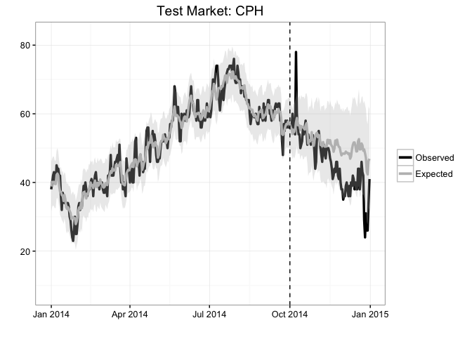
Plot actual observations for test market (CPH) versus the expectation. It looks like CPH deviated from its expectation during the winter:
results$PlotActualVersusExpected
Plot the cumulative impact. The posterior interval includes zero as expected, which means that the cumulative deviation is likely noise:
results$PlotCumulativeEffect

## NULL
Although it looks like some of the dips in the point-wise effects toward the end of the post period seem to be truly negative:
results$PlotPointEffect

## NULL
Store the actual versus predicted values in a data.frame:
pred <- results$Predictions
knitr::kable(head(pred))
| Date | Response | Predicted | lower_bound | upper_bound | |
|---|---|---|---|---|---|
| 2014-01-01 | 2014-01-01 | 38 | 38.82061 | 31.61230 | 46.06123 |
| 2014-01-02 | 2014-01-02 | 40 | 40.15522 | 32.88925 | 46.96195 |
| 2014-01-03 | 2014-01-03 | 42 | 40.12554 | 33.37686 | 47.55353 |
| 2014-01-04 | 2014-01-04 | 43 | 40.18167 | 33.02037 | 47.50588 |
| 2014-01-05 | 2014-01-05 | 40 | 39.56834 | 32.48736 | 46.32851 |
| 2014-01-06 | 2014-01-06 | 40 | 39.52399 | 32.56084 | 46.38276 |
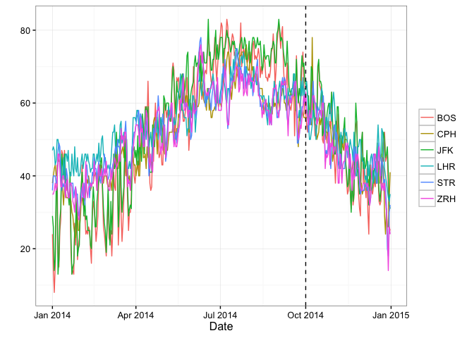
Plot the actual data for the test and control markets:
results$PlotActuals
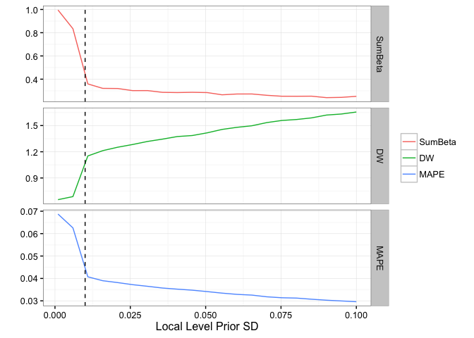
Check the Durbin-Watson statistic (DW), MAPE and largest market coefficient for different values of the local level SE. It looks like it will be hard to get a DW statistic close to 2, although our model may benefit from a higher local level standard error than the default of 0.01:
results$PlotPriorLevelSdAnalysis
Store the average posterior coefficients in a data.frame. STR (Stuttgart) receives the highest weight when predicting the weather in Copenhagen:
coeff <- results$Coefficients
knitr::kable(head(coeff))
| Market | AverageBeta |
|---|---|
| BOS | 0.0071229 |
| JFK | 0.0246569 |
| LHR | 0.0039508 |
| STR | 0.3249443 |
| ZRH | 0.0048855 |
How Does Dynamic Time Warping Work?
Let’s say we have two time series denoted by \(X=(x_1, \ldots, x_n)\) and \(Z=(z_1, \ldots, z_m)\), where \(X\) is the test market (also called the reference index) and \(Z\) is the control market (also called the query index). Note that, although \(m\) and \(n\) do not need to be equal, MarketMatching forces \(m=n\). We’ll denote the common length by \(T\).
In order to calculate the distance between these two time series, the first step is to create the warping curve \(\phi(t) = (\phi_x(t), \phi_z(t))\). The goal of the warping curve is to remap the indexes of the original time series – through the warping functions \(\phi_x(t)\) and \(\phi_z(t)\) – such that the remapped series are as similar as possible. Here similarity is defined by
\[D(X,Z) = \frac{1}{M_{\phi}} \sum_{t=1}^T d(\phi_x(t), \phi_z(t))m_{\phi}(t),\]where \(d(\phi_x(t), \phi_z(t))\) is the local distance between the remapped data points at index \(t\), \(m_{\phi}(t)\) is the per-step weight, and \(M_{\phi}\) is an optional normalization constant (only relevant if \(m \neq n\)). The per-step weights are defined by the “step pattern” which controls the slope of the warping curve (for more details, see [2] as well as the example below).
Thus, the goal is essentially to find the warping curve, \(\phi\) such that \(D(X,Z)\) is minimized. Standard constraints for this optimization problem include:
- Monotonicity: ensures that the ordering of the indexes of the time series are preserved – i.e., \(\phi_x(t+1) > \phi_x(t)\).
- Warping limits: limits the length of the permissible steps. The
MarketMatchingpackage specifies the well known Sakoe-Chiba band (when callingdtw) which allows the user to specify a maximum allowed time difference between two matched data points. This can be expressed as \(\|\phi_x(t)-\phi_z(t)\|<L\), where \(L\) is the maximum allowed difference.
Dynamic Time Warping Example
To see how this works, consider the following example. We’ll use the weather dataset included with the MarketMatching package and use the first 10 days from the Copenhagen time series as the test market and San Francisco as the control market (query series).
Note that the code in this example is not needed to run the MarketMatching package; the package will set it up for you. This is simply to demonstrate the details behind the scene.
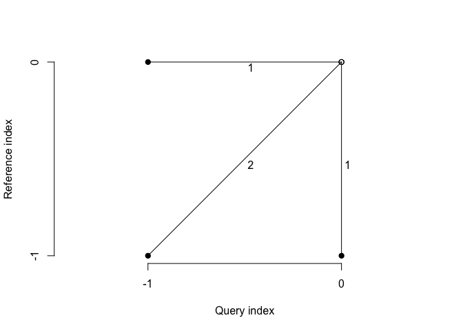
First, let’s look at the warping limits imposed by the Sakoe-Chiba band with \(L=1\):
library(MarketMatching)
library(dtw)
data(weather, package="MarketMatching")

cph <- subset(weather, Area=="CPH")$Mean_TemperatureF[1:10]
sfo <- subset(weather, Area=="SFO")$Mean_TemperatureF[1:10]
cph

##  [1] 38 40 42 43 40 40 45 44 44 42
sfo

##  [1] 49 53 54 55 55 52 54 56 56 54
align <- dtw(cph, sfo, window.type=sakoeChibaWindow, window.size=1, keep=TRUE)
dtwWindow.plot(sakoeChibaWindow, window.size=1, reference=10, query=10)
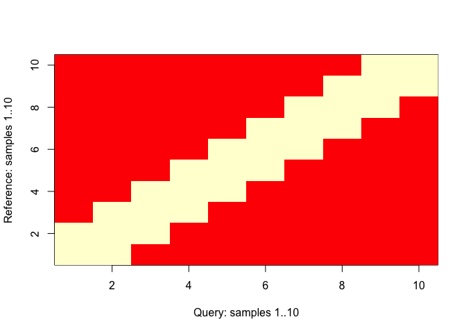
This shows that, as expected, the band is a symmetric constraint around the diagonal. Next, let’s look at the alignment between the two time series. The following code shows the two time series as well as how data points are connected:
plot(align,type="two", off=1)
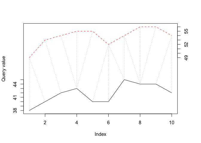
Clearly, the first ten days of these two cities are not well aligned naturally (not surprising given the geographic locations), and that several reference values had to be mapped to three different query values (\(L+1\)is the most replications allowed by the band).
It also helps to look at the actual cost matrix and the optimal alignment path that leads to the minimal distance.
lcm <- align$localCostMatrix
image(x=1:nrow(lcm),y=1:ncol(lcm),lcm,xlab="CPH Index",ylab="SFO Index")
text(row(lcm),col(lcm),label=lcm)
lines(align$index1,align$index2)
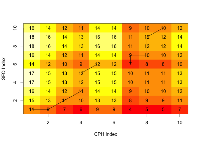
The cells represent the local distances between the two time series. The total cost (distance), \(D(X,Y)\), can be computed by multiplying the distances by their respective weights and then summing up along the least “expensive” path. This can be illustrated by the cumulative cost matrix:
lcm <- align$costMatrix
image(x=1:nrow(lcm),y=1:ncol(lcm),lcm,xlab="CPH Index",ylab="SFO Index")
text(row(lcm),col(lcm),label=lcm)
lines(align$index1,align$index2)
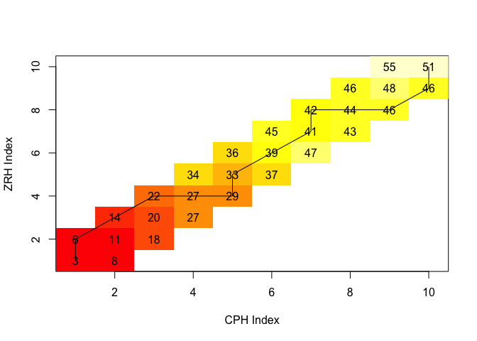
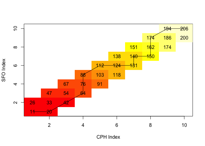 The cumulative distance matrix above shows that minimum (weighted) cumulative distance between Copenhagen and San Francisco equals 206. This is a large number considering that the distance between Zurich and Copenhagen is 51:
zrh <- subset(weather, Area=="ZRH")$Mean_TemperatureF[1:10]
match <- dtw(cph, zrh, window.type=sakoeChibaWindow, window.size=1, keep=TRUE)
lcm <- match$costMatrix
match$distance

## [1] 51
image(x=1:nrow(lcm),y=1:ncol(lcm),lcm,xlab="CPH Index",ylab="ZRH Index")
text(row(lcm),col(lcm),label=lcm)
lines(match$index1,match$index2)
 Recall that the purpose of the dtw algorithm is to find the path that minimizes the total distance, given the constraints and the weights. The weights that are applied to the local distances are determined by the step pattern used. When the default step pattern is chosen, diagonal steps are weighted by a factor of 2 while other steps receive a weight of 1. Thus, with this step pattern a two-step “detour” will cost as much as a direct diagonal step (if all local distances are equal). We can visualize this by using the
 plot function provided by the dtw package:
plot(align$stepPattern)
How Does Intervention Inference Work?
As mentioned, the MarketMatching package utilizes the CausalImpact package written by Kay Brodersen at Google (see [1]) to do the post period inference.
Here’s how it works at a high level:
-
Fit a Bayesian structural time series model using data prior to the pre-intervention period. The model can include the control markets as linear regression components with spike-and-slab priors.
-
Based on this model, generate counterfactual predictions for the post-intervention period assuming that the intervention did not take place.
-
In a pure Bayesian fashion, leverage the counterfactual predictions to quantify the causal impact of the intervention.
This approach has a number of benefits over the “diff in diff” approach: first, using a structural time series model allows us to capture latent evolutions of the test market that cannot be explained by known trends or events. Second, estimating control markets effects with Bayesian priors captures the uncertainty of the relationship between the test market and the control markets. This is critical as it ensures that the counterfactual predictions are not rigidly relying on historical relationships between the test and control markets that may be carrying large standard errors. Moreover the spike-and-slab priors help avoid overfitting by promoting a sparseness during market (variable) selection.
As a result, this approach produces robust counterfactual expectations for the post period that factors in uncertainties in historical market relationships as well as unobserved trends. Moreover, we can calculate posterior intervals through sampling to gauge confidence in the magnitude of causal impact and estimate the posterior probability that the causal impact is non-existent. The “diff in diff” approach does not provide this level of flexibility and does not handle parameter uncertainty nearly as well.
Some Technical Details
When MarketMatching calls CausalImpact the following structural time series model (state space model) is created for the pre-intervention period:
\(Y_t = \mu_t + x_t \beta + e_t, e_t \sim N(0, \sigma^2_e)\) \(\mu_{t+1} = \mu_t + \nu_t, \nu_t \sim N(0, \sigma^2_{\nu})\)
Here \(x_t\) denotes the control markets and \(\mu_t\) is the local level term. The local level term defines how the latent state evolves over time and is often referred to as the unobserved trend. The linear regression term, \(x_t\beta\), “averages”” over the selected control markets. See [1] and [3] for more details.
Once this model is in place, we can create a synthetic control series by predicting the values for the post period and then compare to the actual values to estimate the impact of the event. In order to gauge the believability of the estimated impact, posterior intervals can be created through sampling in a pure Bayesian fashion. We can also compute the tail probability of a non-zero impact. The posterior inference is conveniently provided by CausalImpact package.
Note that the CausalImpact package can fit much more complicated structural time series models with seasonal terms as well as dynamic coefficients for the linear regression component. However, MarketMatching package requests the more conservative model based on the assumptions that the control markets will handle seasonality and that static control market coefficients is sufficient.
About Spike-and-Slab Priors
As mentioned in the overview, we can select the final control markets while fitting structural time series model. The dynamic time warping step pre-screens the markets, while picking the final markets can be treated as a variable selection problem. In the CausalImpact package this is done by applying spike-and-slab priors to the coefficients of the linear regression terms.
Spike-and-slab prior consist of two parts: the spike part governs a market’s probability of being chosen for the model (i.e., having a non-zero coefficient). This is typically a product of independent Bernoulli distributions (one for each variable), where the parameters (probability of getting chosen) can be set according to the expected model size. The slab part is a wide-variance Gaussian prior that shrinks the non-zero coefficients toward some value (usually zero). This helps combat multicollinearity, which is rampant since markets tend to be highly correlated.
This approach is a powerful way of reducing a large set of correlated markets into a parsimonious model that averages over a smaller set of markets. Moreover, since this is a Bayesian model, the market coefficients follow random distributions and we can incorporate the uncertainties of the historical relationships when forecasting as opposed to relying on a rigid encoding based on fixed coefficients.
For more details in spike-and-slab priors, see [1].
How to Select the Local Level Standard Error
There’s no perfectly scientific way of choosing the standard error (SE) of the local level term. Using a pure goodness-of-fit-based measures is not meaningful as a higher SE will always guarantee a better historical fit. In addition, the goal of the model is not to fit the data in the post-intervention period which means that we cannot use the post intervention period as a hold-out sample.
Here are some tips to deciding the size of the standard error:
-
In general, larger values of the standard error leads to wider posterior forecast intervals and hence results are more likely to be inconclusive. Thus, choosing a large value “to be safe” is not always the prudent choice.
-
If you know a priori that the test market series is volatile due to unexplained noise, choose 0.1.
-
Try different values of the standard error, and check the MAPE and Durbin-Watson statistic. The MAPE measures the historical fit and the Durbin-Watson statistic measures the level of autocorrelation in the residuals. This analysis will show the tradeoff between a larger standard error versus fit and ill-behaved residuals. We want to choose a standard error that is as small as possible in order to rely more on the predictive value coming from the control markets, but not at any cost. The
MarketMatchingpackage produces charts that help make this tradeoff. Note that the Durbin-Watson statistic should be as close to 2 as possible. -
When you cannot make a decision, choose 0.01.
Note on Structural Time Series Models
The class of structural time series models deployed by the CausalImpact package provides the most flexible and transparent approach to modeling time series data. In fact, all ARIMA models can be converted into a structural time series model. Take for example the ARIMA(0,1,1) model.
where \(B\) is the backshift operator, \(\rho\) is the AR(1) coefficient, and \(a_t\) denote the residuals. This model can be recast as the structural model with a local level term (the model described above). However, it’s fair to say that the structural model is more transparent and easier to control than the ARIMA model: it is more transparent because it does not operate in a differenced space, and it is easier to control because we can manage the variance of the local level term in a Bayesian fashion.
References
[1] CausalImpact version 1.0.3, Brodersen et al., Annals of Applied Statistics (2015). http://google.github.io/CausalImpact/
[2] Vignette for the dtw package: https://cran.r-project.org/web/packages/dtw/vignettes/dtw.pdf.
[3] Predicting the Present with Bayesian Structural Time Series, Steven L. Scott and Hal Varian, http://people.ischool.berkeley.edu/~hal/Papers/2013/pred-present-with-bsts.pdf.