Seasonal Trends at Stitch Fix

At Stitch Fix, we build tools that help us to delight our clients, which includes performing the thoughtful research that enables such tools. A great example of this is how we study methods for identifying temporal trends. Consider seasonality, which describes the cyclical patterns in how our client’s preferences change over a year. Identifying seasonal trends requires a mixture of time series analysis and machine learning that is challenging but of critical importance to a fashion retail organization. We recently presented some of the methods we have developed to identify seasonal patterns (or other temporal changes that could be induced by the volatile nature of the fashion business) at the Machine learning meets fashion KDD workshop. Here we offer a brief overview of our paper, “Detection of fashion trends and seasonal cycles through the analysis of implicit and explicit client feedback”. We refer the interested reader to the slides of the talk and the paper for a more complete discussion.

Temporal trends in the fashion industry

Understanding how style preferences change with time is of critical importance to a fashion retail organization. Fashion trends can appear cyclically, with styles re-emerging after decades of absence. Fashion preferences can also change on a yearly timescale as a result of changing weather. Other styles become very popular, but then quickly disappear (sometimes for the greater good of humanity). Identifying and anticipating which–if any–of these trends are affecting client preferences can enable more effective control of an organization’s inventory.

Big data and statistical modeling provide a new and powerful method to quantify and test our understanding of fashion trends. However, there is a limited literature about detecting fashion trends using large datasets. One potentially powerful source of relevant data is social media. Studies have examined the content and tags of Twitter and Instagram posts (Manikonda et al. 2015), or have attempted to identify fashion topics on Twitter (Beheshti-Kashi et al. 2015a). Google trends has also been used to identify changes in how types of clothing have been searched (Zimmer & Horwitz 2015). With thousands of fashion blogs and online magazines, the web is full of information about fashion. Aggregating such information could change the way to identify fashion trends (Beheshti-Kashi et al. 2015b).

Leveraging our feedback culture

At Stitch Fix we have a great opportunity to understand fashion trends and seasonal cycles, since our clients give us very explicit feedback about each piece of clothing they encounter. As a client receives a fix with a personalized selection of 5 items that our algorithms and stylists have curated, she has to decide which items to keep. After such a decision, the client goes through a checkout process in which she gives detailed feedback about how the decision was made by filing a multi-option survey where she can provide feedback on fit, size, style and price.

This gave us the idea to attack the problem of seasonality (and fashion trends) in a different way. Rather than anticipating these trends with outside resources, we could identify them using all the feedback collected from the clients, and act accordingly to improve our client’s experience. This should work particularly well for seasonal trends, since by definition they tend to repeat over time, but it should also be possible to detect more subtle shifts in our client’s preferences that could point to overall fashion trends.

One of the great benefits of this approach is that the fashion and seasonal trends detected are extracted from our client behavior, so there is no risk associated with having to extrapolate external sources of trends to our own company. In addition, it has the potential to identify trends in very particular sets of styles, which makes it easier to make the right decisions about when to buy them or place them in the inventory.

In this particular post we will describe how we can use style feedback to understand which of our individual styles are more seasonal and when it is the right time to send the items. For this purpose, we will focus on the style feedback received from our clients.

The setup: from client feedback to temporally aggregated binomial draws

When a client receives a fix, we request feedback about each item. The style feedback for an item takes the following form:

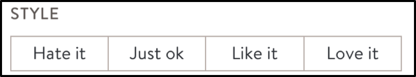
Figure 1. Style feedback form. For each item, we can learn about how much the client loved or hated its style.

In order to simplify the statistical analysis, we transform any feedback obtained from the client into a binary variable, which in this case will be positive if the client likes it or loves it, and will be negative otherwise. We can repeat this process for every style feedback sent by a given client \(C_i\) for a certain style \(S_j\), and create a dataset where we record each binarized style feedback \(Y_{ij}\) in a row, with all the relevant features for the client \(C_i\) and the style \(S_j\), and most importantly, a measure of the time when the feedback was given.

Our method relies on detecting temporal changes in the average feedback given by the clients to a particular style. In principle, we could split our data into several temporal intervals and calculate the average feedback in each one, and associate a certain confidence interval around it based on the normal approximation (see section 3 of the paper). However, this approach comes at a price, since we have to be sure that every temporal interval contains enough feedback interactions to be able to apply the normal approximation, and this becomes even more problematic if we want further divide our data based on client or style attributes.

A simpler method to see how the feedback is changing with time would be to use logistic regression with several time-dependent features. In our case, we have decided to go one step beyond and use Generalized Linear Mixed-effect models (GLMMs, Breslow 93), which have several advantages over logistic regression.

The first advantage is the ability to accept binomial draws as inputs rather than binary variables. Once we have decided which features matter in our model (including time), we can obtain a new aggregated dataset that simply contains the number of positive and negative responses received in each category. For example, in the absence of client features, we aggregate the feedback into weekly (or any other time interval) rows for each different style, which will likely result in a severe reduction of the size of our dataset.

The second advantage is a bit more technical, since it arises from the distinction between fixed and random effects within our GLMM. A simple model could be constructed only with fixed effects, for example having a constant offset for all styles in our dataset. The model would predict the same average feedback for all items at any time. We could then add a categorical variable that has a different level for each style, which would result in a different independent constant prediction for each style. However, in the presence of thousands of styles, with some of them having more feedback from clients than others, it is better to set these offsets as random effects. This still allows each style to have its own offset, but these offsets are now drawn from a Gaussian distribution that is constrained using the data from all styles. One can think about the fixed effect as the average of this distribution, and the random effect as the deviations from this particular average. If we have styles with less feedback, these will always lie closer to the fixed effect value, since the Gaussian distribution acts as a prior for these coefficients. This is similar to some types of regularization used in Machine Learning, that could be also be applied to the logistic regression model described above.

A seasonal trend classifier

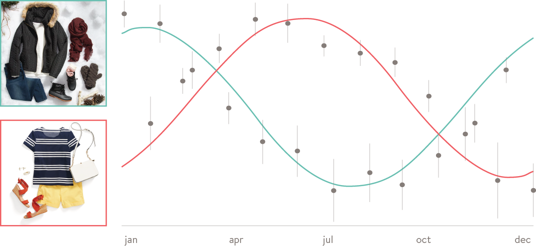
In considering which types of items are seasonal (and to what season they belong), certain patterns seem very clear from looking at what the industry has been doing for a while. For example, sleeveless tops are meant to appear in the shops a bit before the beginning of the summer, and by the time the summer is over, warmer clothes will start appearing on the stores.

To take a first step towards understand seasonality using data, it is useful to make a few simplifying assumptions. All the items that belong to a certain style will receive positive feedback from any given client with a certain probability \(p(t)\) that exclusively depends on the time \(t\). We want this probability to be the same on a particular day of the year, for example it should be the same on June 1st of 2015 and 2016. For that, we can define a timescale \(T\) equal to one year in this case, and make sure that probability \(p(t + T) = p(t)\). Of course, this is simply requiring that the probability function \(p(t)\) is periodic, and the best and simplest example of a periodic function is a sinusoid:

Where \(p_0\) is a constant offset, \(A\) is the seasonal amplitude, and \(t_0\) dictates where the probability is at its maximum. Since we want to use a linear model to describe a general sinusoid, weapply some transformations to describe this periodic probability as:

With this idea in mind, building the classifier becomes a bit easier. We take the dataset with the binomial draws for each week and each style id, and calculate the sine and cosine terms for each week. We then run a GLMM with the following formula

Where both the fixed effect and random effect matrices have coefficients for an offset, a cosine and a sine term. This allows us to obtain individual temporal coefficients for each style in our dataset, and use those coefficients and their confidence intervals to classify them as seasonal or not. In the paper, we used simulations to show that this type of classifier is capable of classifying highly seasonal styles with a very high accuracy, but here we focus on an application to our own data.

Results

We ran our GLMM seasonal trend classifier on the style feedback data for thousands of styles that we have carried over the last few years at Stitch Fix. Unlike in the paper, we were mostly curious to find styles for which we have a very high confidence that they were seasonal. Clearly, newer styles are at a disadvantage, since we have not built enough of a baseline to properly detect trends on them. More common styles will have an advantage, since we will have more feedback data for those.

After we obtained coefficients and confidence intervals for the cosine and sine terms for each style, we looked at the list of 5 styles that had the highest absolute value for the Z-score for either of those terms (defined as the coefficient divided by the margin of error). It is important to note a seasonal style can manifest with a large coefficient for the sine term and a small one for the cosine term, and vice versa, and even in some cases both coefficients could be large. This will depend on the season where the style peaks and the arbitrarily defined zero of our time variable.

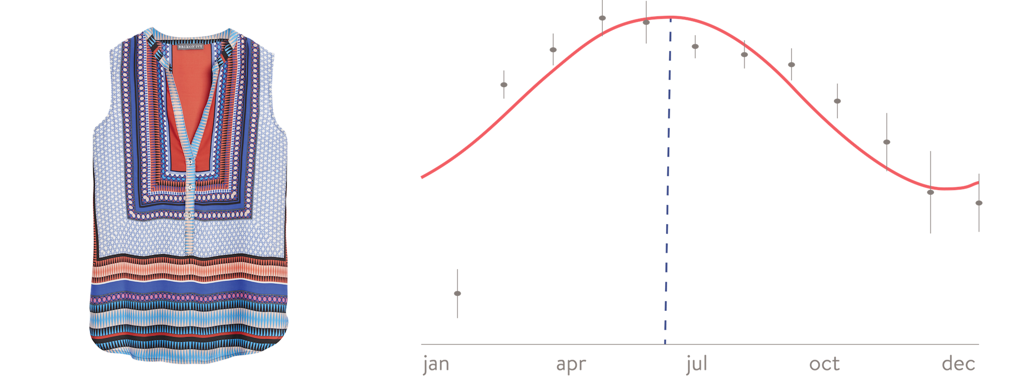
Figure 2. Example of a very seasonal style from our Stitch Fix catalog. The right plot shows how the style feedback from our client (black dots with confidence intervals as bars) changes with the season. The red line is the underlying GLMM model, and the blue line is a visual guide to understand when this style peaks. The left plot shows a picture of the style in question.

We would like to highlight one particular example of a style that describes well how this method works. The style feedback, best fit model and picture for that style can be seen in Figure 2. The first thing to notice is that the style feedback data is clearly changing over different months, with a seemingly sinusoidal shape. It is important to note that our code is looking for such sinusoidal shapes, so other more irregular seasonal patterns may go undetected by our method. Additionally, the GLMM model seems to be doing a great job at fitting the data, and can be trusted to give a more refined measurement of the peak season for this style. In this case this happens to be early June, which is in great agreement with our intuition, since this style is a sleeveless blouse that should work better during the summer.

From identification to understanding

This blog post and the associated paper describe an efficient way to detect seasonal styles using client feedback. However, to fully leverage these insights, it helps to have a causal account of these temporal fluctuations. The depth and breadth of our fashion data lets us answer such questions in ways that few other organizations can imagine, and that helps us to delight our clients.