Update: Be Wrong the Right Number of Times

Who was wrong the right number of times?

In the days and weeks after the election, the Associated Press did not call a winner in Michigan as the race was too close. On November 28, the Michigan Board of State Canvassers finally certified the race as a victory for Mr. Trump. As of this writing, there are still recounts pending but the situation seems stable enough to revisit this question.

There’s wrong and then there’s wrong—the outcome of the election clearly indicates that the model used by FiveThirtyEight (538) was closer to the truth than that of the Princeton Election Consortium (PEC) in terms of the level of uncertainty in the predictions. It’s not by as much as you might think, though.

Predictions and Outcomes

The final pre-election predictions of the Princeton Election Consortium (PEC) and Five Thirty Eight (538) agreed about the most likely winner in each of the fifty states, differing only in the degree of uncertainty in each race. This makes our comparison easy. The incorrectly predicted states were Florida, Michigan, North Carolina, Pennsylvania, and Wisconsin—five in total.

Reproducing the graph from the previous post:

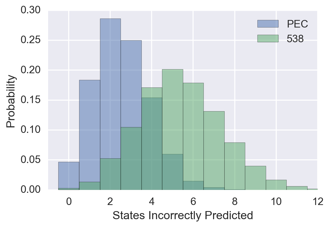
Reading off of the graph, we see that getting five states incorrect is the most likely outcome for 538’s predictions, while it was on the high end of reasonable possibility for the PEC’s model. Based only on the number of states incorrectly predicted, 538’s model is favored over the PEC’s model by a bit better than 3:1 odds.

The Will to (Statistical) Power

This statistical test involving only the number of incorrectly predicted states is useful for discussing the treatment of uncertainty because it’s easy to understand, but it’s probably the weakest test we can we can devise for this case. We could do better by modeling the fifty states as separate terms of a single likelihood function and by taking state-by-state correlations into account.

A quick way to get an idea of what a more detailed analysis might show is to use the output of each model with respect to the national election. This must take into account all of the state-level correlations, and the people who produced each model have almost certainly thought harder about their model than anyone else—certainly harder than I am likely to think about it. This is quite a bit different from the problem we posed above—the overall election winner is determined not by the state results themselves, but rather a sum over the state results weighted by the number of electoral votes for each state.

This is a classic application of Bayes Theorem: it’s easy to calculate the probability that Mr. Trump wins given that 538’s model is correct (538 has kindly done this for us), but now we want to know the probability that 538’s model is correct given that Mr. Trump won the national election. Taking P(Trump wins | 538’s model is correct) = 18 percent and P(Trump wins | PEC’s model is correct) = 1 percent, three lines of algebra allow us to compute the odds ratio:

That is to say the odds are eighteen to one in favor of 538’s model assuming the priors for each model are equal.

These two possibilities are probably upper and lower bounds on reality: 538’s model is favored over the PEC’s model with odds somewhere between 3 to 1 and 18 to 1 (and it’s probably closer to the latter figure). Note that we have just characterized the meta-uncertainty—the uncertainty in the uncertainty—which is a useful thing to get in the habit of doing.

It’s probably a subject of interest to the PEC. There were probably two issues contributing to the fact that their predictions were so far off. The first is correlated error: the distribution of polling results was not centered on the eventual outcome of the election—the mean of the distribution was off. The second is exactly this meta-uncertainty: the width of the distribution of possible outcomes was much wider than the PEC thought.

Would you take that bet?

One concrete way to “ask yourself” if you really believe a probability is correct is to phrase it in terms of a wager. If I really believed that the PEC model was correct, then I should be happy to take make a wager where if Mr. Trump wins I get $2 and if Secretary Clinton wins I pay $100. According to the PEC, Mr. Trump’s chance of winning was 1 percent, so over repeated trials I expect to make $1 per trial on average.

There’s some evidence that Sam Wang, the driving force behind the PEC, would have taken this bet. He famously tweeted that he would eat a bug if Mr. Trump got more than 240 electoral votes, and then followed through.

Let us pause to take this in: what would Professor Wang have gotten if he had won the bet? Not the ability to say “I told you so”; he would have had that anyway. All he would get is the ability to say “I told you so, and I was so sure that I was right that I offered to eat a bug, secure in the knowledge that that would never come to pass.” Against that rather slender gain in the case of a win, consider the outcome in the case of a loss: eating a bug. This sounds pretty close to the proposed bet-$100-to-win-$2 wager proposed above.

Bug eating seems to be Professor Wang’s go-to bet to make a point about his level of certainty. He’s quite thoughtful about it, though, calibrating the level of confidence required to make such a bet to keep his rate of bug eating to acceptable levels. He certainly understands the idea of being wrong the right number of times.

Correlations are Key

Go back to our original proposed statistical test—the number of incorrectly predicted states assuming each state is independent. Suppose the number of incorrect predictions was much higher than the PEC predicted. Is this incontrovertible evidence that the PEC model was wrong? It’s pretty clear the answer is no: the PEC might defensibly say “That’s because your independence assumption was bad: state results are correlated and they were systematically off in one direction—that’s why you think we missed too many states. If you take those correlations into account, the model is fine.”

What if the number of incorrectly predicted states was zero: much lower than 538 predicted. Is that incontrovertible evidence that 538’s model was wrong, or could they make essentially the same claim as above?

Phrased more technically and simplified a bit for clarity: Suppose I make 100 simultaneous bets on the outcome of 100 Bernoulli-type random variables, where the probability of success in any one of them is 50%. So far I’ve specified the mean and diagonal terms of the covariance matrix of the 100 dimensional probability density function. If the random variables are uncorrelated so that all of the off-diagonal terms are zero, then I should be very surprised if I win all 100 bets simultaneously on a single trial. The probability of this is about \( 10^{-30} \). The question: Is there a way to choose the off-diagonal terms of the covariance matrix so that it’s not surprising if I win all 100 bets on a single trial?

My intuition was that correlations could increase the number of incorrect predictions, but not decrease it. This turns out to be wrong—off diagonal terms in the covariance matrix can move the number up or down. This is pretty obvious once you think about it the right way, but it was not my initial intuition.

The right way to think about it to see that this can happen is to imagine that a single underlying random variable controls all 100 of the random variables I defined above. All of these variables are perfectly correlated and the covariance matrix is singular. When the underlying random variable comes up 0, then random variables 1-50 come up 1 and the rest come up 0. Conversely when the underlying random variable comes up 1, then random variables 51-100 come up 1 and the rest come up 0. It will be pretty easy to recognize this pattern and place 100 bets where you either win all of them or lose all of them. In this situation, it would not be surprising at all to either win or lose all of the bets from a single trial simultaneously.

Denouement

Although both models were wrong in predicting the overall election winner, 538’s model was much closer to being wrong the right number of times in the state-by-state election results. The PEC’s model involved too high a level of certainty in the outcome and is disfavored by as much as 18 to 1 odds as a result.

Covariance can turn an extremely surprising result into one that’s not surprising at all. Unmodeled correlations are probably the single biggest factor that make data science difficult by making it hard to come to secure conclusions about causal processes from historical data alone.

Phrasing a statistical result in terms of a wager can be a useful concrete way to ask yourself whether you really believe the number that’s coming out of your analysis. This helps you characterize the uncertainty in your uncertainty: meta-uncertainty.