Introduction
As a proudly data-driven company dealing with physical goods, Stitch Fix has put lots of effort into inventory management. Tracer, the inventory history service, is a new project we have been building to enable more fine-grained analytics by providing precise inventory state at any given point of time, just like the time machine in Mac OSX.
It is essentially a time series database built upon Spark. There are already many open source time series databases available (InfluxDB, Timescale, Druid, Prometheus), and they are more or less designed for certain use cases. Not surprisingly, Tracer is specially designed to reason about state.
Reasoning about state in time series
Inventory evolves over time and every change should be described by an event. It’s natural to model inventory as time series events. However, reconstructing the inventory state at any point in time given these time series events is a challenge.
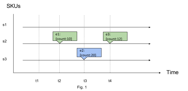
There are two kinds of events: stateful and stateless. Stateful events contain state at a certain point of time. This is a very common type of event. For example, we can have events reporting SKU (Stock Keeping Unit) counts over time, as illustrated in Fig. 1. Another example can be temperature reported by a remote IoT thermometer every 5 minutes.
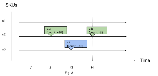
Stateless events contain information about how state changed at the point of time rather than state itself. We can rewrite the previous SKU count example with the changes in counts shown as in Fig. 2. Take a bank account as another example: every transaction event can have either credit or debit to balance, but not the balance itself.
So how can we reason about state at any point of time if we have stateful events? If there exists an event at the time for which we requested, we can directly read the state out of it, otherwise we need to find the last event right before that time to get the state.
If we have stateless events, it becomes a bit tricky as events don’t indicate states directly, therefore we need to establish some initial state as base, then apply the change from the time of that initial state to the time for which we requested to get a new state.
A bit of math
No matter whether we choose to use stateful or stateless events, we can generalize the pattern to reason about state simply with two functions:
- State function
I(tn), returns the state at any point of time tn - Difference function
D(t1,t2), returns the state transition between timet1andt2
These two functions are pure, meaning for a given tn or a tuple of (t1, t2), function I and D will always return the same result. This property is important and gives us confidence that we get the result we expect.
The difference function is especially interesting in that the returned state transition can be in various forms, depending on the use case:
- Time series with current state at each point of time:
(t1, state1) -> (t2, state2) -> (t3, state3)… - Aggregated result in state change
Δstate, such as total credit/debit change for a bank account - Time series with previous state and current state:
(t1, state0, state1) -> (t2, state1, state2) -> (t3, state2, state3)… - Compressed time series between
t1andtn:(t1, state1) -> (tn, staten)
Importantly, the difference function should be aware of the chronological order of state transition, so that if we reverse the input timestamps the returned result should also be in reversed order.
D(t1, t2) = -D(t2, t1)
Once we define the operation to apply a difference to a state, we can reason about state forward and backward.
I(t2) = I(t1) + D(t1, t2)I(t1) = I(t2) - D(t1, t2) = I(t2) + D(t2, t1)
I can not emphasize enough that the difference function D is very flexible. As long as it stays pure and holds true to formulas 1. and 2., it can contain state transition information in any form.
Design
The design of Tracer follows the math foundation described above, which is actually inspired by the MPEG video compression algorithm. Basically the algorithm picks a number of key frames which contain complete information of static pictures at given moments in a video and then encodes changes of motion in between these key frames in a compressed format. When a video player opens an MPEG format video, it decodes the file by using key frames and applying changes in between to restore frame by frame pictures on screen.
Similarly, two building blocks of Tracer, snapshot (green) and delta (orange), are exactly mapped to the state I function and the difference D function to store state and transition data, illustrated in the following graph.
A snapshot contains the complete information of state at a given point of time. If we are going to store SKU count, for example, a piece of snapshot data can look like this.
| as_of_ts | sku_id | warehouse_id | sku_in_count | sku_out_count |
| 20170302 1200 | 1834 | 2 | 1 | 0 |
| 20170302 1200 | 1856 | 2 | 1 | 0 |
| 20170302 1200 | 2441 | 38 | 1 | 0 |
Accordingly, a piece of delta in this case can look like this:
| as_of_ts | received_ts | sku_id | warehouse_id | sku_in_delta | sku_out_delta |
| 20170302 2350 | 2017-03-02 15:57:32 | 74648 | 1 | -1 | 1 |
| 20170302 2350 | 2017-03-02 15:51:50 | 74649 | 1 | 1 | -1 |
| 20170302 2350 | 2017-03-02 15:55:57 | 74730 | 38 | -1 | 1 |
Notice this does not store events directly, rather, it stores the effect caused by events on SKU counts. By doing so, the operation to apply a delta to a snapshot is simply to summarize the sku_in_delta and sku_out_delta and then add up to sku_in_count and sku_out_count respectively for the same time window. As I mentioned before, we can be creative to store events in different ways to best serve the way we use Tracer.
Implementation
Tracer is implemented on top of Apache Spark in Scala and exposed to end users through both Scala and Python APIs. The returned result is just a standard Spark dataframe, so it’s very convenient to connect Tracer to our existing Spark based data pipelines, as well as making it easily queryable through SparkSQL or the dataframe API.
For example, users can query Tracer for inventory state with a timestamp or multiple timestamps. Or more conveniently, they can query with a time window over a certain interval.
from datetime import datetime
from sfspark.sfcontext import AASparkContext
import tracer

aa_spark = AASparkContext("tracer-query-example")
inventory = tracer.Inventory(aa_spark)

# SKU count from 2017-4-14 12:00 to 2017-4-14 14:00, every 15 mins
result = inventory.sku_count_range(
    datetime(2017, 4, 14, 12, 0),
    datetime(2017, 4, 14, 14, 0),
    {"minutes": 15})

result.show()
aa_spark.stop()
AASparkContext is our internal augmented SparkContext with additional helpers. Once you have that, then just initialize a Tracer inventory service object and start sending queries.
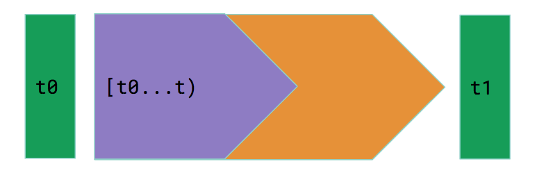
Easy enough? What actually happens under the hood is that for each timestamp requested (for example, at time t), Tracer will check the timestamp and find out the closest snapshot (snapshot at t0 in this case) and apply the correct delta time windows (indicated by the purple part) to the snapshot to build a virtual snapshot, which is exactly the inventory state at the requested timestamp.
Currently snapshot and delta data are stored in S3 just like other spark tables. These implementation details are completely hidden to our end users, enabling us free to later adopt other kinds of data storage, such as Cassandra or in-memory solutions.
This transparency also brings another advantage that we can apply all sorts of optimization under the hood, such as how and where we store the internal data and in what structure, and how we execute a query, all without asking end users to change any code on their side.
One such optimization is indexing. An index is a list of pointers to the locations of snapshots. When Tracer starts planning to run a query, it can quickly identify the location of related snapshots without actually scanning through the contents of other unrelated snapshots.
We originally decided to create snapshot partitions hourly but later realized some delta partitions were huge during rush hours, as we had a lot more events happening within certain hours of a day. With an index, we can distribute data more efficiently by adding snapshot and delta partitions based on data volume instead of a fixed time schedule.
Future work
With two simple core concepts, snapshot and delta, Tracer provides a flexible framework to reason about state with time series data. The scope of Tracer is of course applicable beyond inventory: client events, stylist events … any event we create or consume where we need to understand how state would transition from one to another.
With Tracer it’s even possible to use it for future state! Given a prediction model m, and a timestamp t in the future, a new I(t, m) function can still stay pure by using predicted events. Imagine that!