Are fashion stylists musicians? We think so, even though they may not know it!
Hearing colors
“Synesthesia is a perceptual phenomenon in which stimulation of one sensory or cognitive pathway leads to automatic, involuntary experiences in a second sensory or cognitive pathway” – Wikipedia.
Before meeting a cyberneticist Adam Montandon, a color-blind artist Neil Harbisson used to produce only black-and-white art. Thanks to Harbisson’s collaboration with Montandon and later with Peter Kese a magical device came to be, a device Harbisson calls an ‘eyeborg’. The ‘eyeborg’ transposes the light frequencies of color hues into sound frequencies, allowing him to hear the spectrum of colors even beyond the range of human sight.
Imagine a color-blind Stitch Fix Client. She opens a Fix full of colorful fabrics carefully selected by her personal stylist. How can we enrich her experience so it is not restricted to any perceived range of colors? Borrowing from the ‘eyeborg’ idea, can we present her with a personalized song along with her Fix, that will represent and enhance what her stylist chose just for her? We want to find ways for our Client to experience Synesthesia.
Playing Chords With Fixes
At Stitch Fix, we have many algorithms that predict how likely clients are to buy an outfit, like the style, like the fit, etc. Stylists then leverage the recommendations of the algorithms we produce to assemble your Fix. Combining the algorithms’ suggestions with their own preferences, as well as their experience with the Client, Stylists select 5 fashion items that get sent to the Client. In a normal setting this selection is equivalent to selecting 5 items out of \(C\) classes with replacement, where \(C\) is thousands of possible styles. In order to illustrate our idea for experiencing Synesthesia let’s assume that \(C=88\), which corresponds to the number of keys on a full-size piano.
In order to map from thousands of styles to these 88 classes, we can consider a simplified taxonomy for our items, for instance jeans, knits or shoes. Now we can represent a Fix with a “5-hot” encoding scheme; that is, a binary vector \((y_1, \ldots, y_{88})\) encodes each Fix, where \(y_i =1\) if an item of that category is in the Fix, and \(y_i = 0\) otherwise (see Figure 1).

By now you may have guessed where this is all leading. If we think of each Fix as a chord with up to 5 pitches, then a sequence of Fixes can be thought of as a progression of chords! As music lovers, we were excited to discover a bridge between fashion and music. Are fashion stylists musicians? We think so. Stitch Fix stylists leverage the match-score algorithm to compose Fixes that from our new perspective can be thought as composing music pieces. Analysing the past behavior of thousands Stitch Fix stylists we can now envision a data-driven solution for creating an Artificial Synesthesia.
Mapping Styles to Sounds
Since we want to “hear” Fixes, we need to find a mapping from style categories to musical pitches. There are many methods for representing audio features from music data (see Music Data Analysis). Here, we will try a Histogram, a Pitch Association Matrix, and a Pitch Transition Matrix. For the music, we chose a midi representation of the song “Yesterday” by the Beatles.
A Histogram representation counts the number of times a note occurs. If we count the number of times each style class occurs, we have a similar histogram representation of our Fixes.
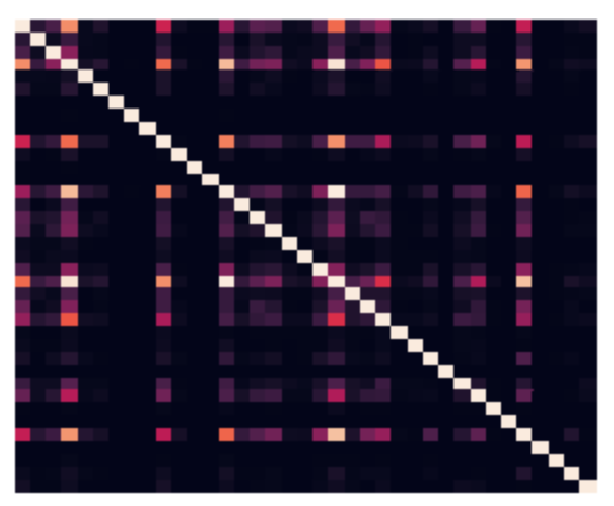
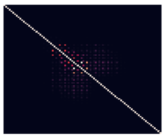
A Pitch Association Matrix \(a_{ij}\) counts the number of times two pitches, \(i\) and \(j\), are played together. We can derive a similar matrix measuring the pairwise association of styles. The normalized Pitch Association Matrices for “Yesterday” and selected Fix sequences are depicted in Figure 2. Since we actually have fewer style categories than pitches, we will truncate the pitches to the most frequently occurring in our training set.


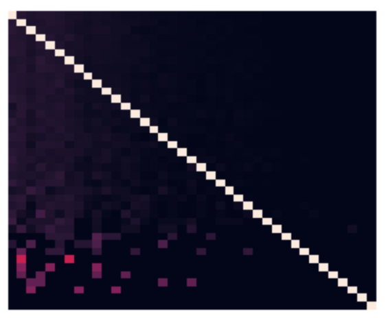
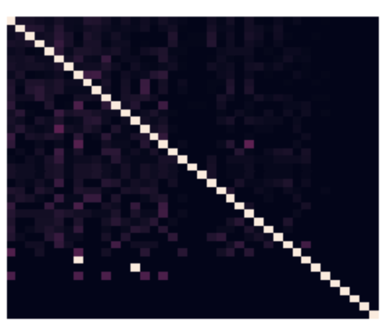
A Pitch Transition Matrix is a Markov Transition matrix where each row \(i\) is a vector (indexed by \(j\)) of probabilities of transitioning from state \(i\) to \(j\). We can build transition matrices for both music and Fixes (see Figure 3).


Algorithmically Finding a Mapping
Mapping with the Histogram is trivial. We just map the most frequently sent style class to the most frequently occurring note, and the second most frequently sent style class to the second most frequently occurring note, and so forth. This approach is computationally straightforward and only requires computing histograms and sorting them. Finding a mapping given Association or Transition Matrices is not quite as straightforward as with Histograms. Given two matrices such as the Style Association Matrix and the Pitch Association Matrix that have the same dimension, \(n \times n\), we can map the style classes to pitches by permuting the Style Association Matrix such that it minimizes some distance measure. A natural choice of between-matrix distance is defined by the Frobenius Norm, i.e.,
\[\Vert A \Vert_2 = \sqrt{\sum_{i=1}^n\sum_{j=1}^m a_{ij}^2}\]which is analogous to the 2-norm of a vector. Our problem can be represented as the following (NP-Hard) constrained non-linear binary optimization problem, similar to the types of problems we routinely solve on the Operations Algorithms team:
\[\begin{align} \min_{P} \qquad & \Vert A - PBP^\intercal \Vert_2^2 \nonumber\\ s.t. \qquad &\sum_i^n p_{ij} = 1, \quad \text{for}\ j = 1, \ldots, n, \nonumber\\ &\sum_j^n p_{ij} = 1, \quad \text{for} \ i = 1,\ldots, n, \nonumber\\ &p_{ij} \in \{0, 1\}, \quad \text{for} \ i, j = 1, \ldots, n \nonumber \end{align}\]where the matrix \(A\) is the Pitch Matrix (either Style or Association), and \(B\) is the corresponding Style Matrix. \(P\) is a row-permutation matrix, which is a matrix containing only zeros and ones, with only a single 1 on each row, and a single 1 on each column. The operation \(PBP^\intercal\) will move rows and columns at the same time. For example if the matrix \(PB\) swaps the first and third rows of \(B\), \(PBP^\intercal\) will swap first and third columns along with the first and third rows.
You may have noticed an issue with the problem as it’s been defined: the function to minimize has fourth order terms in our optimization variables and is therefore highly non-linear and very difficult to solve efficiently. If we pass this problem to the open-source Bonmin solver, you will have to wait a long time for a solution (a pair of \(25 \times 25\) matrices does not finish within a few hours on a Macbook Pro), but even worse, there is no guarantee the solution is a global minimum!
Luckily, we can take advantage of some properties of the Frobenius norm, and the permutation matrix \(P\). After doing some matrix algebra, we find that minimizing the equation above is equivalent to minimizing the following quadratic problem:
\[\begin{align} \min_{P} \qquad& - \text{tr}(PA^\intercal P^\intercal B) \nonumber \end{align}\]If we reshape our matrix \(P\) into the vector \(\mathbf{q}\),
\[\mathbf{q} = q_k = \begin{bmatrix} p_{11} \\ p_{12} \\ \vdots \\ p_{1n}\\ p_{21}\\ \vdots\\ p_{nn} \end{bmatrix}\]then we can rewrite the minimization problem as:
\[\begin{align} \min_{\mathbf{q}} \qquad & \mathbf{q}^\intercal M \mathbf{q} \nonumber\\ M & =A^\intercal \otimes B^\intercal \nonumber\\ s.t. \qquad C\mathbf{q} & = \mathbf{b} \nonumber \\ q_k &\in \{0, 1\} \quad \text{for}\ k = 1, \ldots, n^2 \nonumber \end{align}\]where \(M\) is the Kronecker product of \(A\) transpose and \(B\) transpose, and \(C\) and \(\mathbf{b}\) are simply our original constraints on matrix \(P\) expressed for the vector \(\mathbf{q}\).
The problem has now been simplified to a quadratic binary minimization problem. It’s still NP-Hard and non-linear, but if the matrices \(A\) and \(B\) are both Symmetric Positive Definite (SPD), then the Kronecker product of them is also an SPD matrix, and thus the problem is convex. This is great news for us because now if we pass this problem to Bonmin, the problem solves much faster and, maybe more importantly, we are guaranteed that any local minimum is also a global minimum. We know that both Style and Note association matrices are SPD, so we are ready to roll! On the same Macbook Pro, Bonmin is able to find a solution for a \(40 \times 40\) matrix in a few minutes.
Unfortunately, Transition matrices are not SPD, so we lose these guarantees, but we can give the problem a little nudge in the right direction by assigning 1’s on the diagonals of both matrices. Doing so will make the problem more likely to be convex, while not affecting the outcome since they will not influence the cost of row/column ordering.
The Sound of Style
Now we can compare these 3 mapping methods and see how a sequence of Fixes sounds. We used a single song, “Yesterday” by the Beatles, to determine Pitch Histogram, Association, and Transition Matrices. For generating the Fix representations, we used sequential Fixes received by a few of our longer term clients. We sorted all of the Fixes by time and by client and used them to generate Style Histograms, Associations, and Transition Matrices. Then we picked the history of Fixes from just one client to listen to what their experience with Stitch Fix “sounded” like.
Histogram mapping
Association Matrix mapping
Transition Matrix Mapping
We noticed that the Association Matrix mapping sounds quite similar to the sorted Histogram method. This is probably because they both encode overall note frequency information. Mapping with the Transition Matrices gives us something a little different, with a bit more focus on mid-tone notes. Is it better than using Association or Histogram? We’ll let the listener decide.
Afterword
Following Neil Harbisson’s lead, we might be able to develop a Stitch Fix ‘eyeborg’ that allows users to hear their Fixes as well as see and feel them. The songs could use some more work, and we’ve bounced around some ideas of how we might incorporate different tracks, more temporal information, or volume dynamics. Overall it’s a pretty fun space to play around in!
Moving further, now that we’ve described a method for mapping a stream of Fixes to music, a question naturally arises: can we use music generated by a composer (or maybe a Recurrent Neural Net) and map it back to the styling world? What other fields might we be able to find interesting mapping relationships, and can they help us make better styling decisions? Stay tuned for the Synesthesia part 2 blog post…
Acknowledgements
The authors would like to thank Johnty Wang (McGill University) for his valuable feedback on this blogpost.
