We understand that there is a lot going on in the world right now. We're continuing to publish blog posts in the hope they provide some intellectual stimulation and a sense of connection during these times. See the following for actions that we’re taking regarding racial justice and COVID-19.
Note: this post is based on Optimal Testing in the Experiment-rich Regime, which is joint work with Ramesh Johari and Virag Shah.
A core aspect of data science is that decisions are made based on data, not (a-priori) beliefs. We ship changes to products or algorithms because they outperform the status quo in experiments. This has made experimentation rather popular across data driven companies. The experiments most companies run today are based on classical statistical techniques, in particular null hypothesis statistical testing. There, the focus is on analyzing a single experiment that is sufficiently powered. However, these techniques ignore one crucial aspect that is prevalent in many contemporary settings: we have many experiments to run and this introduces an opportunity cost: every time we assign an observation to one experiment, we lose the opportunity to assign it to another.
We propose a new setting where we want to find “winning interventions” as quickly as possible in terms of samples used. This captures the trade-off between current and future experiments and gives new insights into when to stop experiments. In particular, we argue that experiments that do not look promising should be halted much more quickly than one would think, an effect we call the paradox of power. We also discuss additional benefits from our modeling approach: it’s easier to interpret for non-experts, peeking is valid, and we avoid the trap of insignificant statistical significance.
An illustrative example
Before diving into the setting more formally, we think it’s illustrative to consider the following example. Suppose you are a high school baseball coach trying to recruit new players to your successful team. There’s a large group of interested freshmen that are eager to join the highly rated team, and you can’t possibly test all skills of each player. You also know from experience that most students lack the skills to join the team. Instead, you want to make a first cut by focusing on batting, so that you can then spend more time with a much smaller group to make your final picks.
Consider the first phase; selecting players that are sufficiently adept at batting. You have the recruits form a long line, and start pitching the ball to the first player in line. After each throw, based on performance, you have three choices:
- You can pitch another ball to the same student to get more information about the player’s skill.
- You can reject the player from consideration because they are not good enough, and move on to the next player.
- You can accept the player as good enough to make it to the next round, and move on to test the next player.
Your elbow has seen better days and the kids easily lose patience. How would you decide on the most effective approach to find 20 promising players while limiting the amount of pitches it takes? That is, use the fewest amount of pitches to discover 20 great players with low error rate.
We set up a simulation of the scenario below, where you step into the role as coach. In this case, we are looking for players that have a batting average above 0.4, and we don’t want to mistakenly accept players with a lower batting average with probability exceeding 10%. The batting average of each player is drawn from a Beta(1, 2) distribution. [1]
Also play around with simple automated policies: we added a fixed sample size policy where the coach pitches a fixed number of balls to each player, and an early stopping policy that stops whenever a student’s batting average is above 0.4 with 90% confidence (a success) or below a threshold you set (and we move on to the next student). How effective are these?
(homage to xkcd)
Notice that the fixed sample size policy, where each batter gets a fixed number of throws, is horribly inefficient. You spend way too many pitches on players who are obviously terrible, or clearly good enough. As a result, if you adopt this policy, you definitely need a new elbow and can’t coach the team in the upcoming season.
In comparison, the early stopping policy does much better. This policy stops throwing pitches whenever it thinks a player is not good enough, or, to the contrary, clearly is good enough. However, if you run the policy a couple of times, you notice that sometimes it gets stuck on a player that is right on the border of good enough. It takes an enormous amount of pitches to figure out whether this player should make the cut. From a fairness perspective, we might want to find out exactly how good this player is, but it’s terrible from an efficiency standpoint, and for your elbow![2]
Experimentation
It may seem that the above thought experiment has little to do with experimentation, but for modern applications I beg to differ. Nowadays, many companies run hundreds, if not thousands of experiments every week. Especially in web technology, it has become trivial to test many alternatives. Thus, we can think of all the experiments we want to run as baseball trials, and we’re interested in finding as many successful interventions as quickly as possible.
You may be skeptical: can’t we run multiple experiments at the same time? And don’t we have so much data nowadays that we can test all the things without running into sample size issues? Unfortunately, those cases are not as common as we would like. In particular, experiments could clash in ways that make it impossible to run them at the same time, or they could interfere with each other, making it more difficult to do inference, especially as the number of concurrent experiments grows. Thus, there are benefits to limiting the number of concurrent experiments. And while it’s true that there is more data than ever, that doesn’t necessarily solve our problems: effect sizes are often small and there are many things to test. As the scale of a company grows, even small effects can translate to large absolute changes in dollars. However, we often need a lot of data to detect meaningful changes in an experiment.
Aiming for discoveries
Suppose there is an infinite stream of experiments. Without loss of generality, we focus on policies that consider experiments sequentially. We collect observations sequentially and after every sample (or batch of samples), we either declare a positive result for the current experiment, continue assigning observations, or give up and move on to the next experiment. Because there is always a next experiment lined up, there is a natural cost to continuing with the current experiment as it delays learning about the next one.
Since there is an infinite stream of experiments, we model this from a Bayesian viewpoint. We can use the previous experiments as a guide to use as prior for future ones. As an added benefit, Bayesian posteriors satisfy two of the desired properties that frequentist testing struggles with. First, they are much easier to explain to non-experts. Second, there is no need to correct them for continuous monitoring; they are “always valid” by design.
Our final ingredients are a desired effect size and error rate, both set by the experimenter. For example, the goal might be to find an intervention that improves a specific metric by X and we want to be 95% sure that we don’t make a mistake when we declare an intervention a success.
Now the goal is to find as many successful interventions in the shortest amount of time (measured in observations). Equivalently, we want to find an experimentation policy that minimizes the expected time to find the first successful interventions (at which point we can restart the process).[3]
Let’s make this a bit more formal; we consider a sequence of interventions indexed by \(i\). Each intervention has an unknown mean effect that we want to estimate, denoted by \(\mu_i\). Based on past experiments, we assume that each mean effect is independently drawn from a prior distribution: \(\mu_i \sim P\) (the prior is known). For each intervention, we then sequentially observe samples \(X_1, X_2, X_3, \ldots\) drawn from a distribution parameterized by \(\mu_i\), and decide either to obtain another sample, or reject the current experiment and start a new one.
Definition of a discovery
The data scientist decides on a desired effect threshold \(\theta\) and a tolerance level \(\alpha\) (e.g. \(\alpha = 0.05\)). Then, we say that the intervention is a discovery after \(t\) samples if the posterior probability that \(\mu_i > \theta\) is greater than \(1-\alpha\):
\[\mathbb{P}(\mu_i > \theta \mid X_1,X_2,\ldots, X_t) > 1-\alpha\]Note that this condition is both similar and different to the frequentist type-I error condition: it’s a parameter that sets a level of accuracy required. Let \(T\) be the first time the above condition holds for some intervention \(i\), then we want to choose our actions to minimize its expectation, \(\mathbb{E}[T]\).
Exploration
Given the above model, the question is how to go about deciding whether to obtain an additional observation, or move on to a new intervention? Unfortunately, we do not have a closed-form expression for the optimal solution; in the paper mentioned above we discuss a way to approximate it by solving a dynamic program. The dynamic program uses the expected time to reach the next discovery as a value function to decide which action is optimal. In particular, we compare the expected time if we restart from scratch with the expected time until discovery if we take another sample for the current experiment. If the latter is shorter, then we keep sampling for the current experiment.
However, the main property of an optimal policy is easy to state and actionable: stop interventions aggressively if they don’t look promising. The idea is simple: discoveries ought to be rare (if they aren’t, then you should probably be running more experiments![4]) This means that in order to be efficient, it is important to stop non-discoveries as quickly as possible so that we can test the next experiment. If not, then too many observations are wasted, delaying a discovery.
Interventions whose effect is close to the discovery threshold are especially dangerous, as we could be spending an arbitrarily large number of observations to learn on which side of the threshold they fall. It’s much better to give up on these and hunt for interventions whose effect is clearly larger than the threshold, which will generally require fewer observations to discover.
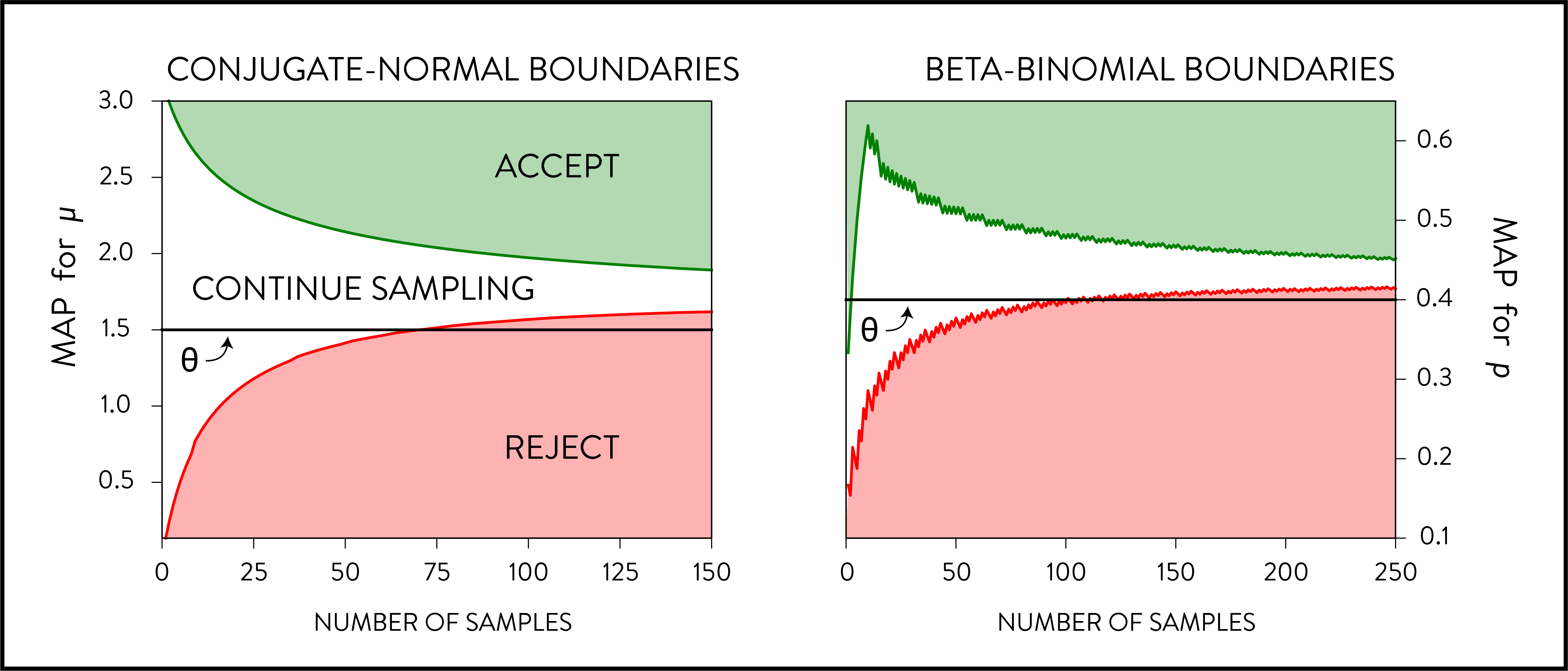
An efficient experimentation platform thus stops interventions quickly if they aren’t promising, and focuses most of its observations on experiments that look promising. The figure illustrates the the optimal boundaries for rejection in terms of the maximum a posteriori (MAP) estimate for two standard experimental settings where the effect threshold, \(\theta\), is denoted by the black line. On the left, we consider the case where observations are drawn from a normal distribution and we have a normal prior on the mean, while on the right observations are Bernoulli draws and the prior is a Beta distribution. Once the MAP hits the green area, we can declare the intervention a discovery. If the MAP hits the red area, we should stop and move on. If neither hold, then we should continue gathering observations.
These are computed by solving the dynamic program (see paper). In particular, note that the rejection boundary crosses the threshold; even though the MAP estimate suggests that the intervention is larger than the threshold, it would take too long to verify this to sufficient degree. For example, consider the conjugate normal case with threshold \(\theta = 1.5\) in the left figure below. If, after 150 samples, the MAP for it is 1.51, then we would reject this experiment despite it being larger than the threshold.
Paradox of power
Recall that one can think of power as the probability of detecting a “true discovery”; that is, if the effect of an intervention is above (or, more extreme than) the threshold, power defines how likely it is that we indeed discover the intervention. If you run fixed sample size experiments, important advice is to power your experiment correctly. That is, make sure you gather enough data to be able to detect an (interesting) effect with high probability. Aiming for 80% power seems to be a common rule of thumb.
Naively, you might then think that high power is desirable in the sequential setting; don’t we want to make many discoveries? But this turns out to be false. One salient feature of efficient policies is the paradox of power: to find many discoveries, you need a procedure that is unlikely to detect true discoveries (i.e. has low power). Procedures that have high power inherently spend too much time on interventions that are not sufficiently promising, leading to a great loss in efficiency and therefore fewer discoveries. Instead we should aggressively discard interventions even if that means that sometimes we discard “true discoveries”.
Conclusion
The internet era has made data-driven decision making easier, faster, and better than ever before. With it come unique challenges and the possibility to rethink how to optimally experiment. We propose a Bayesian setting that implicitly captures the opportunity cost of having multiple interventions to test. Good policies are characterized by two properties. First, they are sequential, and hence adaptive. For some experiments you want to gather many observations, while other experiments should be stopped sooner rather than later. Second, policies that have high power are inefficient as they spend too much time making sure an experiment is not an improvement, rather than moving on to test the next intervention.
Of course, the proposed approach does not solve every problem; each company faces unique challenges when conducting experiments; there is no one size fits all solution. At Stitch Fix, we often have to deal with temporal effects, delayed feedback and physical constraints in terms of inventory that require us to adapt tests to our needs. Rather, the intention is to shed a new light on a problem we’re all familiar with. We believe that the underlying principles of opportunity costs and the paradox of power can guide us towards strategies that lead to finding more discoveries in a shorter time frame.
“All models are wrong, but some are useful” -George Box
[1]↩ These values are chosen so that it’s relatively easy to find good players rather than to realistically model batting
[2]↩ As hinted at, this example ignores the fairness consideration and rather focuses on the statistical problem. This is problematic when deciding which student gets to play on the baseball team, but less so when deciding on the lay-out of a webpage.
[3]↩ There are other natural objectives, for example finding big effects rather than finding effects quickly. It turns out that the latter naturally finds big effects too, because they are the quickest to find (in terms of observations required to detect). As hinted at, this example ignores the fairness consideration and rather focuses on the statistical problem. This is problematic when deciding which student gets to play on the baseball team, but less so when deciding on the lay-out of a webpage.
[4]↩ If most of your experiments are successful, then you might be too conservative in trying new ideas.