At Stitch Fix, when we want to understand the impact of some treatment or exposure, we often run an experiment. However, there are some questions we cannot answer via experimentation because it is operationally infeasible or because it doesn’t feel client-right. For example, we wouldn’t experimentally require stylists to style at specific times of day (most of our stylists work flexible, self-scheduled hours) or experimentally subject clients to poor inventory conditions. In those cases, we rely on observational analysis. The key challenge in this setting is that the treatment has not been randomly assigned, which means that we may have issues with confounding (for more on causal structures, see this previous blog post). Our goal is to learn something true and be as precise as we can; a t-test is not going to cut the mustard here.
One common approach to the challenge of confounding is to use a regression model to estimate the effect of the treatment,
including confounders as covariates. Unfortunately, for a regression estimator to do its job properly, you have to specify
the model correctly. If you fail to specify the model correctly (misspecification), you may think you are fully controlling
for confounders when you are not[1].
Another way to tackle this is to do inverse probability of treatment weighting, where you focus your regression efforts
on learning the probability of treatment. But this modeling task suffers from the same risk - misspecification -
and isn’t terribly efficient. We rarely have a clear understanding of the potentially complex relationship between
covariates, treatment/exposure, and outcomes and yet many of us make unilateral model specifications daily (YOLO?).
Enter: double robust estimation. This class of estimators explicitly acknowledges our human frailty when it comes to correctly specifying the relationships between exposure/treatment, covariates, and outcomes. As luck (errr math) would have it, these methods give us some wiggle room to make a few mistakes and still come out with a consistent estimator. And if you don’t have model misspecification, these estimators are as efficient as it gets[2]. The goal of this post is to demonstrate both the superiority of double robust estimators and the low overhead to using them. For more background, see our previous post on what makes a good estimator.
The TL;DR
- One model is used to estimate the conditional probability of treatment (i.e. the propensity score)
- Another model is used to estimate how the exposure/treatment and other covariates are associated with the outcome
- These models are combined in specific fancy ways to produce an estimate of the target parameter. Understanding the particulars of this requires knowing a bunch of stuff about influence functions and empirical process theory that many of us are not familiar with. We’re gonna stand on the shoulders of giants here and let that lie.
- Here’s the kicker, only one of the two models needs to be correctly specified in order to achieve a consistent estimator[3] of the target parameter. This is where the “double” in “double robust” comes in. Note that not all estimation procedures that use two such models are double robust.
We are going to focus on a method called Targeted Maximum Likelihood Estimation (TMLE) for the purposes of this post but there are other double robust methods including Augmented Inverse Probability Weighting (AIPW) and Generalized Random Forests (GRF).
Before we go on, some quick vocabulary housekeeping:
-
Y: outcome
-
A: binary exposure (in the case of a non-randomized exposure) or binary treatment (in the case of an experiment)
-
W: set of covariates that are predictive of Y or are potential confounders
-
E(Y A, W): This is the conditional expectation of the outcome Y given A (the treatment/exposure) and covariates W -
\( P(A = 1 \mid W) \): This is the probability of treatment/exposure given W, also known as a propensity score. For a randomized experiment, this may be known and independent of W.
- Target Parameter: This is the thing you’re trying to estimate. We are not always formal about this in data science but we’re often implicitly after the Average Treatment Effect (ATE). The terminology ATE is not familiar to everyone, but if you’ve ever run an A/B test and calculated the difference in average outcome between the two cells assuming all else equal, you were estimating the ATE! The ATE can be thought of as the difference between the average outcome if everyone in the data set had been exposed and the average outcome if no one had been exposed, holding all else equal.
A simulated example
We’re going to do a simulation study comparing three different estimators of the ATE using R:
- Two-sample comparison of means performed with a t-test
- Generalized Linear Model (GLM)
- TMLE (Targeted Maximum Likelihood Estimator, doubly robust)
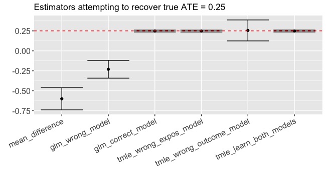
We will simulate a data-generating process with an exposure for which the we know the true ATE and see how well each method estimates the target parameter. In this simulation, the true ATE = 0.25 and the probability of treatment is a function of some covariates. The outcome is a function of both the treatment and the same covariates, which means that there is confounding:
\[\begin{align} W_1 & \sim N(0, 1)\\ W_2 & \sim N(0,1)\\ A & \sim \text{Bernoulli}( \theta ), \text{ where } \theta = f(W_1 + W_2 + W_1*W_2) \in (0.05, 0.95)\\ \epsilon & \sim N(0, 0.2)\\ Y &= 0.25*A - W_1 - W_2 - W_1*W_2 + \epsilon\\ \end{align}\]The function f(.) above is a simple scaling function mapping continuous values to the unit interval (see simulation code below)[4].
If we were analyzing this in the most naive way possible, we might just do a t-test on the difference of means between the exposed group (A = 1) and the unexposed group (A= 0).
mean_diff <- mean(dat$Y[dat$A==1]) - mean(dat$Y[dat$A==0])
ttest_out <- t.test(x=dat$Y[dat$A==1], y=dat$Y[dat$A==0])
Result: -0.60 (-0.74, -0.46)
Yikes! Recall that the true ATE = 0.25. We’re VERY confident in an estimate that doesn’t even have the right sign! This is a great example of when confounding biases the naive estimate.
Ok, next up, a generalized linear model (GLM). We know \(W_1\) and \(W_2\) are confounders. In a main terms regression model \(Y \sim A + W_1 + W_2\), we interpret the coefficient on A as the impact on Y of A=1 compared with A=0, holding \(W_1\) and \(W_2\) constant. In other words, it’s an ATE estimator. Many of us have been trained to start with this kind of main-terms model when we lack specific knowledge about the functional form of the relationship between Y and A,W.
glm_out <- glm(Y~A+W1+W2, data=dat)
glm_coef <- summary(glm_out)$coefficients
glm_ci <- confint(glm_out)
Result: -0.23 (-0.34, -0.12)
Feeling a little sweaty. What we just did is not an uncommon approach to estimation, yet we are still getting the sign wrong (-0.23 instead of 0.25!!) and we are pretty confident about our result (p < 0.001). This is the result of model misspecification. A correctly specified GLM that contains the \(W_1*W_2\) interaction would have given us an unbiased estimate. The question is, how often would we have known that \(W_1*W_2\) was an important interaction? If we had many more covariates, would we feel comfortable specifying a model with all their interactions? Probably not. And for that matter, can a GLM even describe the true relationships that we face when we leave toy-data-land? Many of us were trained to be parsimonious in model specification but here is an example of where it bites back.
OK, time to bring in a double robust method (TMLE). When we use the R package tmle, we have the opportunity to estimate the propensity score and outcome model more flexibly using machine learning via the SuperLearner package. SuperLearner uses generalized stacking to create an optimally weighted combination of diverse sub-models. The weights are a function of cross-validated risk. The sub-models could include different glm specifications, splines, and other machine learning prediction algorithms such as generalized additive models (GAMs), elasticnet regression, etc… Using SuperLearner is a way to hedge your bets rather than putting all your money on a single model, drastically reducing the chances we’ll suffer from model misspecification.
A little note about what we are specifying in the tmle function:
-
Y = outcome
-
A = exposure/treatment
-
W = the matrix of covariates we plan to use
-
Q.SL.library = the sub-models (AKA “learners”) SuperLearner will use to estimate the outcomes model, i.e. \( E(Y \mid A, W) \)
-
g.SL.library = the sub-models (AKA “learners”) SuperLearner will use to estimate the propensity score, i.e. \( P(A \mid W) \)
-
Qform = an opportunity to specify the functional form of the outcomes model (optional). If this is specified, SuperLearner will not be used and this specification will be used in a GLM.
-
gform = an opportunity to specify the functional form of the exposure model (optional). If this is specified, SuperLearner will not be used and this specification will be used in a GLM.
-
V = the number of cross-validation folds for SuperLearner to use
First, suppose we let tmle estimate the outcome model (Y~A,W) using SuperLearner but we will deliberately misspecify the functional form of the exposure model to put the double robustness to the test by omitting the interaction between \(W_1\) and \(W_2\). Recall that only one of these models needs to be correctly specified in order to get a consistent estimator:
tmle_incorrect_exposure_model <-
tmle(Y=dat$Y
  ,A=dat$A
  ,W=dat[, c("W1", "W2")]
  ,Q.SL.library=c("SL.glm", "SL.glm.interaction", "SL.gam", "SL.polymars")
  ,gform="A~W1+W2"    #note: this is incorrect, A is also a function of  W1*W2
  ,V=10
)
tmle_incorrect_exposure_model_ATE = tml_incorrect_exposure_model$estimates$ATE$psi
tmle_incorrect_exposure_model_CI = tml_incorrect_exposure_model$estimates$ATE$CI
Boom. 0.25 (0.24, 0.26)
Daaaaaaaang! First, let’s note that the estimate is almost smack-dab equal to the true value of 0.25. Second, are you seeing that confidence interval? It’s the size of a baby’s toenail clipping! Contrast that to the GLM confidence interval (ignoring for a moment its complete lack of validity) with a width more like a meatball sub. Recall that we got this glorious estimate despite the fact that we deliberately misspecified the exposure model.
Let’s try something else. In the last case, we misspecified the exposure model but used SuperLearner to (probably) correctly specify the outcome model. Let’s try the reverse, let’s use SuperLearner to hopefully correctly specify the exposure model and we’ll deliberately misspecify the outcome model, again omitting the interaction.
tml_incorrect_outcome_model <- tmle(
   Y=dat$Y
   ,A=dat$A
   ,W=dat[, c("W1", "W2")]    #note: recall the correct form contains the interaction of W1 and W2
   ,g.SL.library=c("SL.glm", "SL.glm.interaction", "SL.gam", "SL.polymars")
   ,Qform="Y~W1+W2"
   ,V=10
)
tmle_incorrect_outcome_model_ATE = tml_incorrect_outcome_model$estimates$ATE$psi
tmle_incorrect_outcome_model_CI = tml_incorrect_outcome_model$estimates$ATE$CI
Result: 0.26 (0.12, 0.39)
Much bigger confidence interval this time - but the estimate is very close to the true ATE of 0.25.
Let’s see what happens when we let SuperLearner take care of ALL of the modeling decisions so that we hopefully have two correctly(ish) specified models:
tmle_learn_both_models <- tmle(Y=dat$Y
  ,A=dat$A
  ,W=dat[, c("W1", "W2")]
  ,Q.SL.library=c("SL.glm", "SL.glm.interaction", "SL.gam", "SL.polymars")
  ,g.SL.library=c("SL.glm", "SL.glm.interaction", "SL.gam", "SL.polymars")
  ,V=10
)
tmle_learn_both_models_ATE = tmle_learn_both_models$estimates$ATE$psi
tmle_learn_both_models_CI = tmle_learn_both_models$estimates$ATE$CI
Result: 0.25 (0.24, 0.26)
A thing of beauty, truly.
In a world where we are still specifying the structure of glms by hand, TMLE provides a nice safety net. But what really supercharges this method is the ability to take advantage of all kinds of fancy predictors (nonparametric models, machine learning methods, etc…) when modeling E(Y|A,W) and P(A=1|W). These methods may not even be interpretable on their own which makes them challenging to use for inference. But luckily, TMLE doesn’t require their interpretability, it just requires their predictions. So these more nuanced predictions can be dumped into TMLE and out pops a potentially better estimate of our target parameter benefiting from local efficiency.
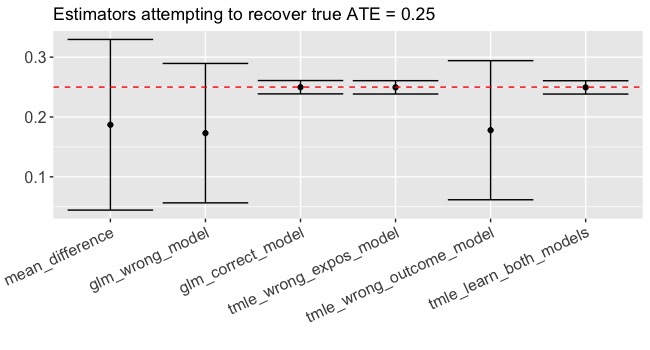
We’ve demonstrated that TMLE can be really handy when we’re worried about confounding. But what if we’re not? What if we’re working with a randomized treatment? It turns out we can still benefit from this methodology because in addition to being doubly robust, it’s also locally efficient which means making the best bias variance trade-off for the thing you actually care about, the target parameter, as opposed to making the best bias variance trade-off for the whole conditional expectation.
Let’s make the same methodological comparison on an exposure that’s been randomized (more commonly called a treatment). In this case, all of the methods are consistent estimators given the data generating process but using the combination of tmle and SuperLearner to estimate efficiently and avoid misspecification leads to smaller confidence intervals (Figure 2). Again, if we correctly specify the functional form in the glm, we do practically just as well but not better than tmle. So using TMLE won’t hurt and it might help!
Sign me up!
Hopefully we’ve convinced you that there are major advantages to using double robust estimation techniques in terms of consistency and efficiency. We’ve also demonstrated that the overhead to execute these more advanced methods is minimal. There are existing packages in both R (tmle) and Python (zEpid). If you want to better understand the mechanics of TMLE in particular, we highly recommend this very accessible paper which goes through the calculations “by hand” without relying on package infrastructure.
Here are some of scenarios in which we use this methodology at Stitch Fix:
- Estimating the ATE of some exposure in observational data where we are concerned about confounding and potentially complex interactions (this is the first case we discussed). We saw that it is possible to do just as well with a glm when reality is simple and we nail the model specification. But why risk it?
- Estimating the ATE of treatment that was randomly assigned, but not uniformly randomly assigned, P(A =1) is not constant for all observations. We can specify known propensity scores or even learn them! We were going to have to do something fancy here anyway, why not be doubly robust?
- Estimating the ATE of a treatment that was uniformly randomly assigned (simple A/B test). Even though it’s not necessary to do anything special to address probability of treatment in this case, we can still benefit from the local efficiency as we saw in the randomized example. This gives us better power for free!
Odds and Ends
A few more things that might come in handy!
Suppose you happened to know the exact propensity scores P(A|W) because you ran an experiment where you controlled the probability of treatment (regardless of whether it was fixed or dependent on W). You can supply that information with the argument g1W instead of supplying a model specification or list of SuperLearner libraries for the propensity score.
tmle_known_propensity_scores <- tmle(Y=dat$Y
  ,A=dat$A
  ,W=dat[, c("W1", "W2")]
  ,Q.SL.library=c("SL.glm", "SL.glm.interaction", "SL.gam", "SL.polymars")
  ,g1W = dat$pA,
  ,V=10
)
Suppose your observations are not independent but instead clustered within subjects in some way. You can specify a subject_id in order to correct for this dependence so that your standard errors are not overly optimistic:
tmle_dependent_obs <- tmle(Y=dat$Y
  ,A=dat$A
  ,W=dat[, c("W1", "W2")]
  ,Q.SL.library=c("SL.glm", "SL.glm.interaction", "SL.gam", "SL.polymars")
  ,g.SL.library=c("SL.glm", "SL.glm.interaction", "SL.gam", "SL.polymars")
  ,id = dat$subject_id
  ,V=10
)
Resources:
Targeted maximum likelihood estimation for a binary treatment: A tutorial
Targeted Maximum Likelihood Estimation: A Gentle Introduction
Code
library(tmle)
library(SuperLearner)
library(gam)
library(polspline)
library(ggplot2)
# ---------------------------
# simulation functions
#----------------------------
# function to bound probabilities
boundx <- function(x, new_min, new_max){
  old_min <- min(x)
  old_max <- max(x)
  stretch_me <- (new_max-new_min)/(old_max-old_min)
  stretch_me*(x-old_min) + new_min
}

# observational data generating process
simple_simdat <- function(rseed, n, true_ate){
  set.seed(rseed)
  W1 <- rnorm(n)
  W2 <- rnorm(n)
  pA <- boundx(W1+W2+W1*W2, new_min=0.05, new_max=0.95)
  A <- rbinom(n, 1, pA)
  epsilon<- rnorm(n, 0, .2)
  Y <- true_ate*A - W1 - W2 - 2*W1*W2 + epsilon
  data.frame(W1=W1, W2=W2, pA=pA, A=A, Y=Y)
}

# randomized data generating process
simple_random_simdat <- function(rseed, n, true_ate){
  set.seed(rseed)
  W1 <- rnorm(n)
  W2 <- rnorm(n)
  pA <- sample(c(0,1), size = n, replace = TRUE)
  A <- rbinom(n, 1, pA)
  epsilon<- rnorm(n, 0, .2)
  Y <- true_ate*A - W1 - W2 - 2*W1*W2 + epsilon
  data.frame(W1=W1, W2=W2, pA=pA, A=A, Y=Y)
}
Complete code available on github.