What makes a good estimator? What is an estimator? Why should I care? There is an entire branch of statistics called Estimation Theory that concerns itself with these questions and we have no intention of doing it justice in a single blog post. However, modern effect estimation has come a long way in recent years and we’re excited to share some of the methods we’ve been using in an upcoming post. This will serve as a gentle introduction to the topic and a foundation for understanding what makes some of these modern estimators so exciting.
What the heck is an estimator?
First let’s start with the target parameter - this is the thing you want to know, the thing you are hoping to estimate with data. It is also sometimes called the estimand. An estimator is a function that takes in observed data and maps it to a number; this number is often called the estimate. The estimator estimates the target parameter. You interact with estimators all the time without thinking about it - mean, median, mode, min, max, etc… These are all functions that map a sample of data to a single number, an estimate of a particular target parameter. For example, suppose we wanted to estimate the mean of some distribution from a sample. There are lots of estimators we could use. We could use the first observation, the median, the sample mean, or something even fancier. Which one should we use? Intuitively, the first option seems pretty silly but how should we choose between the other three? Luckily, there are ways to characterize the relative strengths and weaknesses of these approaches.
What makes a good estimator?
First let’s think about the qualities we might seek in an ideal estimation partner, in non-technical language:
“Open-minded data scientist seeking estimator for reasonably accurate point estimates with small-ish confidence intervals. Prefer reasonable performance in small samples. Unreactive to misunderstandings a plus.”
That’s what we often want, anyway. This brings up one of the first interesting points about selecting an estimator: we may have different priorities depending on the situation and therefore the best estimator can be context dependent and subject to the judgement of a human. If we have a large sample, we may not care about small sample properties. If we know we’re working with noisy data, we might prioritize estimators that are not easily influenced by extreme values.
Now let’s introduce the properties of estimators more formally and discuss how they map to our more informally described needs. We will refer to an estimator at a given sample size n as \(t_n\) and the true target parameter of interest as \(\theta\).
Unbiasedness
The expectation of the estimator equals the parameter of interest:
\[E[t_n] = \theta\]This seems sensible - we’d like our estimator to be estimating the right thing, although we’re sometimes willing to make a tradeoff between bias and variance.
Consistency
An estimator, \(t_n\), is consistent if it converges to the true parameter value \(\theta\) as we get more and more observations. This refers to a specific type of convergence (convergence in probability) which is defined as:
\[\displaystyle \lim_{n\to \infty} P(| t_n - \theta| < \epsilon ) = 1\]This is sometimes referred to as “weak convergence” because we’re not saying that the limit of \(t_n\) is \(\theta\). When something converges in probability, the sampling distribution becomes increasingly concentrated around the parameter as the sample size increases.
Whoa whoa whoa. So what is the difference between unbiasedness and consistency? They kind of sound the same, how are they different? A quick example demonstrates this really well.
Suppose you’re trying to estimate the population mean (\(\mu\)) of a distribution. Here are two possible estimators you could try:
-
The first observation, \(X_1\)
-
The sum of the observations, divided by (n+100), \(\frac{\sum X_i}{n + 100}\)
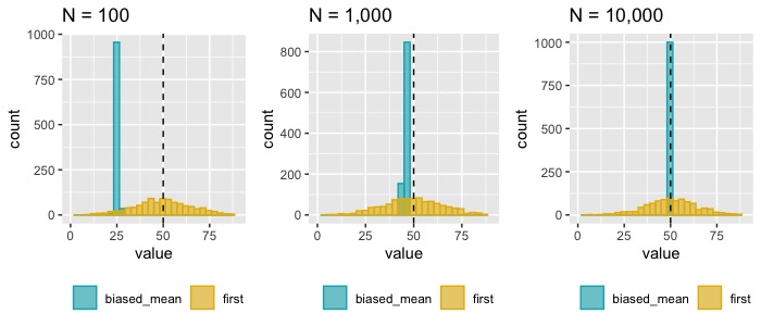
\(E[X_1] = E[X_i] = \mu\), so that estimator is unbiased! But it seems like an intuitively bad estimator of the mean, likely because your gut is telling you it’s not consistent. Taking bigger and bigger samples does nothing to give us greater assurance that we’re close to the mean.
On the other hand, that second estimator is clearly biased: \(\begin{align} E \left[ \frac{\sum X_i}{n + 100} \right] &= \frac{1}{n+100}\sum E[X_i] \\ &= \left(\frac{n}{n+100} \right) \mu \\ &\neq \mu \\ \end{align}\)
But! As n increases, \(\frac{n}{n+100} \rightarrow 1\). So the second estimator is consistent but not unbiased (in fact, it’s asymptotically unbiased). From this vantage point, it seems that consistency may be more important than unbiasedness if you have a big enough sample (Figure 1). Both consistency and unbiasedness are addressing our need to have an estimator that is “reasonably accurate”.
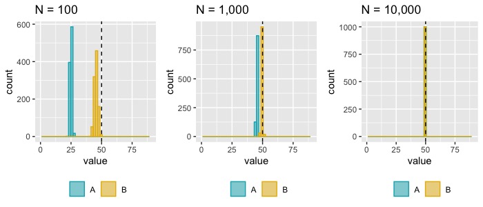
One differentiating feature even among consistent estimators can be how quickly they converge in probability. You may have two estimators, estimator A and estimator B which are both consistent. But the rate at which they converge may be quite different. All else being equal, we’d prefer the estimator which converges in probability most quickly because that gives us better reliability under non-infinite sample sizes, which is the reality most of us inhabit (Figure 2).
Asymptotic normality
We say an estimator is asymptotically normal if, as the sample size goes to infinity, the distribution of the difference between the estimate and the true target parameter value is better and better described by the normal distribution.
This is probably bringing back whiffs of the Central Limit Theorem (CLT). In one of its most basic forms, the CLT describes the behavior of a sum (and therefore a mean) of independent and identically distributed (iid) random variables. Suppose you have iid samples \(X_1, ...X_n\) of the random variable \(X\) distributed according to an unknown distribution D with finite mean m and finite variance v (i.e. X ~ D(m, v)). The CLT for the sample mean (\(\bar{X}\)) tells us that \(\sqrt{n} (\bar{X} - m)\) converges in probability to \(Normal(0,v)\). We can rearrange this to show that \(\bar{X} \rightarrow Normal(m, v/n)\). Some version of the CLT applies to many other estimators as well, where the difference between the estimator \(t_n\) and the true target parameter value \(\theta\) converges to a 0-centered normal distribution with some finite variance that is scaled by the sample size, n.
You might not have even known you wanted this property in an estimator but it’s what you need (wow, that dating profile analogy is really taking flight here). Remember how you wanted small confidence intervals? Asymptotic normality is the underpinning that allows you to use the standard closed-form formulas for confidence intervals at all. We are able to use the formula estimate +/- 1.96*standard_error to produce confidence intervals because we know we have a normal limiting distribution, which allows us to determine the multiplier on the standard error (1.96 for a 95% confidence interval).
Asymptotic normality is not necessarily required to characterize uncertainty - there are non-parametric approaches for some estimators that don’t rely on this assumption. And in fact, asymptotic normality is dependent not just on the estimator but on the data generating process and the target parameter as well. Some target parameters have no asymptotically normal estimators. But in situations where asymptotic normality applies, taking advantage of it will generally produce confidence intervals which are smaller than their non-parametric counterparts and isn’t it a treat to have one that you can do with a pencil?
Efficiency
An estimator is said to be “efficient” if it achieves the Cramér-Rao lower bound, which is a theoretical minimum achievable variance given the inherent variability in the random variable itself. This is true for parametric estimators, the nonparametric crew has other words for this but the overall idea is the same; let us not get dragged into that particular fray. In practice, we are often concerned with relative efficiency, whether one estimator is more efficient (i.e. has a smaller variance) than another.
Let’s take a step back and recall the typical formula for a confidence interval from a second ago (estimate +/- 1.96*standard_error). The asymptotic normality is what allowed us to construct that symmetric interval, we got the 1.96 from the normal quantiles. The estimate is the number we got from our estimator. But where does the standard error in that formula come from?
The standard error we use in the confidence interval has three major drivers:
- the number of observations, n
- the inherent variance of the data generating process itself, i.e. Var(X)
- the variance associated with the particular estimator being used, i.e. the Var(\(t_n\)). Recall that the variance of a function of random variables is different than the variance of the random variables themselves.
We want the standard error to be small because that gives us tighter confidence intervals. There’s usually not much we can do about the variation in the random variable - it is what it is. And if the data has already been collected, we don’t get to choose the n either. But what we DO have control over is the choice of estimator and a good choice here can give a smaller overall standard error which gives us smaller confidence intervals. (Note: this is one of the most important points of this whole blog post)
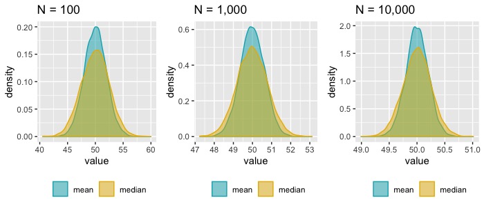
Suppose that we have a sample of data from a normal distribution and we want to estimate the mean of the distribution. Let’s consider two choices, the sample mean and the sample median. Both are unbiased and consistent estimators of the population mean (since we assumed that the population is normal and therefore symmetric, the population mean = population median). You can see in Plot 3 that at every sample size, the median is a less efficient estimator than the mean, i.e. estimates from repeated samples have a wider spread for the median.
The mean/median comparison is a somewhat trivial example meant to illustrate the concept of efficiency but in practice we are not often choosing between those two estimators. A more relevant example is the difference between analyzing an A/B test with a traditional t-test approach compared with a regression model that includes baseline (pre-treatment) covariates. The motivation for using a regression model to analyze an otherwise tidy, randomized experiment is variance reduction. If our outcome has many drivers, each one of those drivers is adding to the variation in the outcome. When we include some of those drivers as covariates, they help absorb a portion of the overall variation in the outcome which can make it easier to see the impact of the treatment.
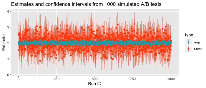
Suppose we have a simple A/B test with a randomly assigned treatment and two pre-treatment covariates that affect the outcome. We could choose whether to analyze the data with a difference in sample means approach or with a regression model that includes those two known pre-treatment covariates. Figure 4 shows the estimates and confidence intervals from 1000 such simulated trials. Both methods are producing valid confidence intervals which are centered around the true underlying effect, but the confidence intervals for this particular simulation were more than 6x wider for the sample mean approach compared with the regression approach.
In this toy example, we had an unrealistically easy data generating process to model. There was nothing complicated, non-linear, or interacting in the data generating process therefore the most obvious specification of the regression model was correct. In a randomized experiment, the model doesn’t necessarily have to be perfectly specified in order to take some advantage of the variance reduction. However, when the treatment is not randomized misspecification of the model could lead to an inconsistent estimator of the treatment effect.
Robustness
Robustness is more broadly defined than some of the previous properties. A robust estimator is not unduly affected by assumption violations about the data or data generating process. Robust estimators are often (although not always) less efficient than their non-robust counterparts in well behaved data but provide greater assurance with regard to consistency in data that diverges from our expectations.
A classical example is a scenario where we are taking smallish samples from a skewed distribution, which can generate outliers. In this case the mean may be a poor estimator of central tendency because it can be strongly influenced by outliers, especially in a small sample. In contrast the median, which is considered a robust estimator, will be unperturbed by outliers.
Another example pertains to an assumption that we often make, which is that the variance associated with a particular variable is the same across all observations (homoskedasticity). This often comes up in the context of regression, where we assume that the values of \(\epsilon_i\) in \(y_i = \beta X_i + \epsilon_i\) are independent and identically distributed. If the latter condition does not hold (e.g. the variance of epsilon depends on \(X_i\)), the standard approach to estimating the standard errors for the \(\beta\) coefficients will be incorrect and probably overly optimistic. The Huber-White or Sandwich estimator of the standard error is a robust estimator designed to provide a consistent estimate under these circumstances which generally results in wider confidence intervals. Safety first!
Conclusion
Now we know what a target parameter is (the thing you want to estimate from the data), what an estimator is (a function that maps a sample to a value), and the properties we might seek in an estimator. We’ve also covered how and where we’re taking advantage of these properties.
Let’s revisit the original request for an estimator and translate between the casual and the technical:
- “reasonably accurate point estimates” \(\rightarrow\) consistent
- “small-ish confidence intervals” \(\rightarrow\) asymptotically normal, high relative efficiency
- “unreactive to misunderstandings about reality” \(\rightarrow\) robust
The final question, why should you care? Estimation is fundamentally a search for truth, we’re not doing this for kicks. In a search for truth, it’s important to know what trade-offs you’re making and whether those are wise trade-offs in the context of your data. Recall that performance across these properties is a tango between the estimator and the data generating process, which means you need to know something about the data you’re working with in order to make good decisions. You should also know what you’re leaving on the table that you could have had for free. If you have pre-treatment covariates that are predictive of your outcome, why use the mean as your estimator and live with wider confidence bounds than you have to? We’ve only scratched the surface here; in a future post, we’re excited to talk about double robust estimation which offers strengths in consistency, efficiency, and robustness.