What Color Is This, Part 2: The Computational Parts
We have to find the colors of our clothes from their images, as we described in our last post about color. This will help us in many ways, including deciding what styles to buy and which clients to send them to. We described the hybrid human-computer approach, but only went into depth about the human part: translating our images into a hierarchy of colors. In this post, we’ll get into depth about the computational part: our current computer vision algorithm, some of our process in coming up with that algorithm, and ideas for what we’ll do next.
How will we know if it’s working?
Before even developing an algorithm, we have to think about how to evaluate it. If we make an algorithm and it says “this image is these colors”, is it right? What does “right” mean?
For this task, we decided on two important dimensions: correct labeling of the main color, and correct number of colors. We operationalize this as the CIEDE 2000 distance (as implemented in scikit-image) between the main color our algorithm predicted and our ground truth main color, and mean absolute error on the number of colors. We decided on these for a few reasons:
- They are easy to evaluate.
- If we had more metrics, it might be difficult to pick a “best” algorithm.
- If we had fewer metrics, we might miss an important distinction between two algorithms.
- Many clothing items only have one or two colors anyway, and many of our processes rely on the main color. Therefore, getting the main color correct is much more important than getting the second or third colors correct.
What about ground truth data? We have labels provided by our merchandising team, but our tools only allow them to select a broad color like “grey” or “blue”, not an exact value. These broad colors encompass a lot of items, so we can’t use them as the ground truth. We have to build our own data set.
Some of your minds might be jumping to Mechanical Turk or other labeling services. But we don’t need very many images, so describing the task might be harder than just doing it. Plus, building the data set helps us understand our data better. Using a quick and dirty bit of HTML/Javascript, we randomly selected 1000 images, picked out a pixel representing the main color of each, and labeled how many distinct colors we saw. Now it’s easy to get two numbers (mean CIEDE distance of main color, and MAE on number of colors) that tell us how well an algorithm does.
At times we also did some manual verification by running two algorithms on the same image and displaying the item with both lists of colors. We then manually rated about 200 of them, selecting which list of colors is “better.” This kind of engagement with the data is important, not only to get a result (“algorithm B is better than A 70% of the time”) but to understand what’s happening in each one (“algorithm B tends to select too many clusters, but algorithm A misses out on some very light colors”).
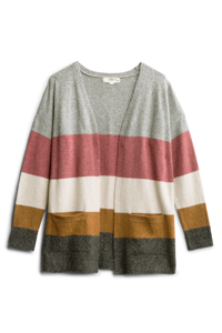
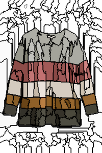
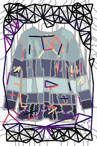
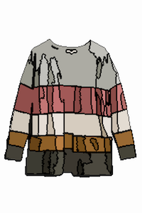
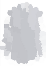
A sweater (center), and two different algorithms' color extraction results (left and right)
Our color extraction algorithm
Before processing our images, we convert them to the CIELAB (or LAB) color space, instead of the more common RGB. Instead of three numbers representing the amount of red, green, and blue in an image, LAB points (technically L*a*b*, though we will call it LAB throughout this post for simplicity) represent three different axes. L represents lightness, from black (0) to white (100). A and B represent the color in two parts: A ranges from green (-128) to red (127) and B ranges from blue (-128) to yellow (127). The main benefit of this color space is its approximate perceptual uniformity: two LAB points with the same Euclidean distance between them will appear approximately equally distinct, no matter where in the space they live.
Of course, LAB introduces other difficulties: notably, images are always viewed on computer screens, which use device-dependent RGB color spaces. Also, the LAB gamut is wider than the RGB gamut, meaning that LAB can express colors that RGB cannot. This means that LAB-RGB conversions are not bi-directional; if you convert points from LAB to RGB and back, you probably will not get the exact same points. We acknowledge that these are theoretical shortcomings in the rest of this work, but empirically it works.
After we convert to LAB, we have a series of pixels, which can be seen as (L, A, B, X, Y) points. The rest of our algorithm is two-stage clustering on these points, where the first stage clusters based on all 5 dimensions, and the second stage omits the X and Y dimensions.
Clustering using space
We start with an image of a flat item that has been color corrected as described in the previous post, shrunk to 300x200, and converted to LAB.
First, we use the Quickshift algorithm to cluster nearby pixels into “superpixels.”
This already takes our image from 60,000 pixels to a few hundred superpixels, removing a lot of unnecessary complexity. We can even further reduce these superpixels by merging nearby ones that are close to the same color. To do so, we draw a regional adjacency graph over these superpixels: a graph where two superpixels are connected if their pixels touch.
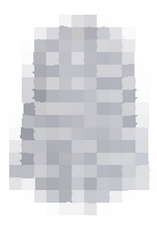
Left: the Regional Adjacency Graph (RAG) on this cardigan. Dark lines between two superpixels show that there is not much difference between the superpixels' colors, and therefore they can be merged. Bright lines (or no lines) suggest that there is a high difference between these colors and therefore they should not be merged. Right: the superpixels, merged after thresholding on the RAG.
The nodes of this graph are the superpixels we computed before, and the edges are the difference in color space between the superpixels. Two nearby superpixels that are very similar colors will have low weight (corresponding to dark lines in the image), while superpixels that are very different colors will have high weights (bright colors, or not even drawn in this image if the edge weight is greater than 20). There are many ways to figure out how to combine nearby superpixels, but we’ve found that a simple threshold of 10 works well.
Now, in this case, the 60,000 pixels have been reduced to about 100 regions, where each pixel within a region has the same color. This has some nice computational benefits: first, we know the background is that big superpixel that’s almost pure white and we can easily remove it. (We remove any superpixel where L > 99 and A and B are both between -0.5 and 0.5.) Second, we can greatly reduce our pixels to cluster in the next step. We can’t reduce them to just 100, because we want to weight regions based on the number of pixels in them. But we can safely delete 90% of the pixels from each cluster without losing much detail or skewing our next clustering step too much.
Clustering without using space
At this point, we have a few thousand (L, A, B) pixels. There are many methods that can neatly cluster these pixels; we went with K-means because it runs quickly, it’s easy to understand, our data has only 3 dimensions, and Euclidean distance in LAB space makes sense.
We’re not being very clever here: we simply cluster with K=8. If any clusters contain fewer than 3% of the points, we try again with K=7, then 6, and so on. This gives us a list of between 1 and 8 cluster centers and fractions of how many points are part of each center. We add names to them using colornamer, as described in our previous post.
Results and remaining challenges
We’ve achieved a mean CIEDE 2000 distance of 5.86 between the predicted color and our ground truth colors. Giving a good interpretation of that number is tricky. By a simpler distance metric, CIE76, our mean distance is 7.82; on that metric, 2.3 corresponds to a just noticeable difference. So we could say our results are a little over 3 just noticeable differences away.
We also have a MAE of 2.28 on the number of colors. Again, this is a far secondary metric. Many of the other algorithms described below (notably, the gap statistic) reduce this error, but at the cost of an increase in first color distance. It’s much easier to ignore spurious 5th and 6th colors than it is to ignore a wrong 1st color.
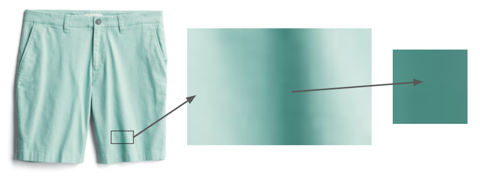
Even items that are clearly only one color, like these shorts, contain areas that appear to be much darker, because of shadows.
Shadows remain a problem. Because fabric never lies perfectly flat, there is always some portion of an image that remains in shadow and therefore spuriously appears to be a separate color. Simple approaches like deduping colors with similar hues and different lightnesses don’t work because the transformation from “unshadowed pixel” to “shadowed pixel” isn’t always consistent. In the future, we hope to use some more clever techniques like DeshadowNet or Automatic Shadow Detection to remove them.
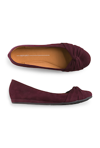
We’ve only focused on apparel images so far. Jewelry and shoes pose problems: our jewelry photos are very small, and our shoe photos often contain the inside of the shoe. In the example above, we would label this shoe as burgundy and sienna, though only the burgundy is important.
What else we tried
While our final algorithm seems straightforward, it wasn’t straightforward to come up with! In this section, we’ll detail a few of the variations we tried, and learned from, along the way.
Background removal
We’ve tried algorithms for background removal, such as this one from Lyst. Informal evaluation showed that they weren’t as precise as just removing white backgrounds. However, we plan to dig deeper into this as we do more processing of images that our photo studio hasn’t processed!
Pixel hashing
A few color-selection libraries have implemented a very simple solution to this problem: cluster pixels by hashing them into a few broad buckets, then return the average LAB values of the buckets with the most pixels. We tried a library called Colorgram.py; despite its simplicity, it works surprisingly well. It also works quickly: under 1 second per image, as opposed to tens of seconds for our algorithm. However, Colorgram’s mean distance from the main color was larger than our existing algorithm, mostly because its results are averages of big buckets. Nevertheless, we still use it for cases when speed is more important than accuracy.
Different superpixel algorithms
We’re using the Quickshift algorithm to segment the image into superpixels, but there are many possible algorithms, such as SLIC, Watershed, and Felzenszwalb. Empirically, we had the best results with Quickshift, due to its results with fine details. SLIC, for example, seems to have trouble with features like stripes that take up a lot of space in a not-very-compact way. Here are some representative results from SLIC with various parameter values:
| Original Image | compactness=1 | compactness=10 | compactness=100 |
|---|---|---|---|
|
|

|
|
Quickshift has one theoretical advantage for our data: it doesn’t require that its superpixels are completely connected. Researchers have noted that this can cause problems, but in our case, it’s a benefit, because we often have small detailed areas that we want to all be the same cluster.
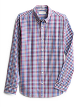
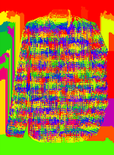
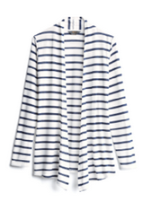
A plaid shirt (left), and Quickshift superpixel clustering applied to that shirt (right).
(While the superpixel clustering looks like a complete mess, it’s really grouping all the red lines in this shirt with other red lines, blue lines with blue lines, etc.)
Different methods for numbers of clusters
When using K-means, one common question is, “what should K be?” That is, if we want to cluster our points into some number of clusters, how many clusters should we have? A number of solutions have been developed. The simplest is the Elbow Method, but that requires manually looking at a graph, and we want a fully-automated solution. The Gap Statistic formalizes this method, and using it we got better results on the “number of colors” metric, but at the cost of some accuracy on the main color. Because the main color is more important, we haven’t put it into production, but we plan to investigate more. Finally, the Silhouette Method is another popular method for selecting K. It also produces results slightly worse than our existing algorithm, and has one major shortcoming: it requires at least 2 clusters. Many articles of clothing only have one color.
DBSCAN
One potential solution for the question of “What should K be?” is to use an algorithm that doesn’t require you to specify K. One popular example is DBSCAN, which looks for clusters of similar density in your data.
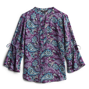
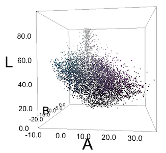
Left: a multicolored blouse. Right: each pixel in the image on the left, plotted in LAB space. Notice that, unfortunately, the pixels do not form clear "teal" and "purple" clusters.
Often we don’t have these clusters, or we have things that only look like clusters because of human perception. To our eyes, the teal buta elements in the garment on the left pop out from the purple background, but when we plot each pixel in RGB or LAB space, they don’t form clusters. Still, we tried DBSCAN, with various values of epsilon, but got predictably lackluster results.
Algolia’s solution
One good research principle is to see if anyone has solved your problem already. In fact, Léo Ercolanelli at Algolia posted an in-depth solution on their blog over three years ago. Thanks to their generous open-sourcing, we were able to try out their exact solution. However, we got slightly worse results against our ground truth data set, so we stuck with our existing algorithm. They’re solving a different problem than we currently are: pictures of merchandise on models with non-white backgrounds, so it makes sense that we would have slightly different outcomes.
Color Coordination
This algorithm completes the process we described in our previous post. After we extract these cluster centers, we use Colornamer to apply names, then import these colors to our internal tools and algorithms. This currently helps us easily visualize our merch by color; we hope to include it in our recommendation systems for buying and styling as well. While this process isn’t a perfect solution, it helps us get much better data about our thousands of merch items, which in turn improves our ultimate goal: helping people find the styles they’ll love.