This blog post has been adapted from an article that will appear in an early 2017 special issue of Revista Indice dedicated to research and development in statistics. The journal is edited by the Autonomous University of Madrid in collaboration with the National Institute of Statistics of Spain.
At first sight the difference between planets outside our solar system (exoplanets from now on) and fashion trends seems enormous, but all of us math lovers know that entirely different phenomena can have an almost identical mathematical description. In this very peculiar case, exoplanetary systems and certain fashion trends can be characterized as having a periodic nature, with certain magnitudes repeating cyclically, and this will allow us to use very similar techniques to study them.
Hunting exoplanets using the transit technique
During the last two decades, scientists from all over the world have discovered thousands of planets outside our solar system. The transit technique is the most successful one used to find them, and it is based on detecting a temporary drop in the measured brightness of a star during an eclipse (the so called transits). During a transit, the planet blocks part of the star’s surface because it passes in front of it from our point of view, generating the described drop (check out this video with more a detailed explanation, with yours truly as a supporting actor).
This technique exploits the fact that the planet’s orbit has an associated temporal scale (the orbital period \(P\)), such that the planet passes in front of the star every P days. Seeing a planet transit its host star several times at the right times gives credibility to the planet’s discovery, and most of the algorithms used to detect these signals take advantage of this periodicity. The shape of the signal depends on the relative size between the planet and the star, and also on the orbital velocity and orientation with respect to the equator of the star.
The connection with the world of fashion
A large number of industries are currently being disrupted by companies that have been capable of obtaining and studying large amounts of data generated by their clients. If you read this blog frequently, you are probably aware that Stitch Fix is a data driven personalized e-commerce company, that uses a humans-in-the-loop data driven approach to optimize our clients’ experiences. This focus on personalization requires a deep understanding of our clients’ preferences.
Methodologies used to discover exoplanets become relevant when investigating how clients’ preferences change with time. Some of these preferences tend to repeat every year, so they can be studied in a very analogous way to detecting transiting exoplanets, and we can use this type of analysis to anticipate those preferences and make decisions to improve our service.
Generating the Fourier spectrum in the case of a transiting exoplanet
There is not a more elegant way to study the shape of a periodic signal than by constructing its Fourier spectrum, which helps us to visually identify the most important periodicities that describe the signal. We can use that to detect transiting planets, but first we need to obtain a time-series of observations of a star’s brightness. These observations will have a true physical component that we want to detect but also an associated uncertainty, which is assumed to be Gaussian distributed since the number of photons that the telescope’s detector receive per observation is generally quite high.
When these observations are taken at equidistant times ti, a set of equations can be applied to obtain the Discrete Fourier Transform of the signal, and one can even speed up the process by calculating a Fast Fourier Transform. However, in Astronomy it is rarely the case where the equidistance constraint applies, so the way to obtain the Fourier transform is a bit different. What is used is known as the Lomb-Scargle Periodogram, which builds a frequency spectrum by fitting a series of sinusoidal functions to the data for each periodicity \(P\), with a fixed form
\[f(t) = a \sin{\left(\frac{2 \pi t}{P}\right)} + b \cos{\left(\frac{2 \pi t}{P}\right)} \]At a fixed value of \(P\), for each entry in the time-series at a time ti we can calculate the sinusoidal terms and use a linear least square model to fit the data and obtain the values of \(a\) and \(b\). A plot that shows how \(a^2 + b^2\) as a function of the periodicity \(P\), or the frequency \(1/P\), allows us to evaluate the periodic part of our signal in a direct and visual way.
A Fourier spectrum adapted to our clients behavior
One of the most direct ways for us to evaluate our client’s preferences is by simply listening to them. During the ordering process, our clients are allowed to write a short note describing what they are looking for, so that our stylist can personalize their fixes as much as possible.
In a previous blog post we already explained how we can obtain interesting information from these request notes, but to save time, we essentially use NLP techniques to identify topics that appear frequently in different requests notes, particularly when they are mentioned with positive intent.
The next step is to construct two time-series, calculating first the amount of times, \(N(t)\), that our clients have written a request note for a fix on a given day, and within those request notes, identify how many times, \(n(t)\), we have identified a particular topic being mentioned in a positive way. The fraction \(n(t)/N(t)\) can already be used to show how the probability that a given client requests clothes that are connected with a given topic changes with time.
To approach this as a tractable statistical problem, we can understand this process as having a set of \(N(t)\) independent clients that are faced with the choice of asking, or not asking, about a particular thing with a certain probability \(p(t)\) of actually asking for it. This means that the quantity \(n(t)\) is binomially distributed as opposed to Gaussian distributed, which was the assumed distribution for our exoplanet data. Fortunately, we can still use the same method to build a new type of Fourier spectrum, in which we fit the same sort of sinusoidal functions to our data, but using a generalized linear model (GLM). This type of model is far more flexible, accepting input variables from a wide range of distributions from the exponential family, and the final Fourier spectrum built this way will represent the periodic component of the time-dependent function \(p(t)\).
Letting the data speak
Let’s put in practice the described techniques with real data. The chosen planet is Kepler-78b, the first planet that I discovered in graduate school, which was actually identified from the shape of its Fourier spectrum. With an orbital period of 8.5 hours, the planet completed approximately 3000 orbits during the four years in which Kepler was able to observe its host star in an almost continuous way. On the upper left corner of the main figure of this blog post we can see the Fourier spectrum of the data downloaded from the NASA archives using the kplr python package. The highest peak on the Fourier spectrum has a frequency of approximately 3 cycles per day (which is the number of orbits that the planet completes in a day). The other peaks appear at exact multiples of this principal frequency, and they always appear when the periodic component of a signal cannot be described with a single sinusoidal function. Once we have identified the principal frequency, we can use it to fold all 3000 orbits, binning all observations into a super light curve, that has a lower scatter and allows us to see the presence of the planet’s transits (see lower left part of the figure).
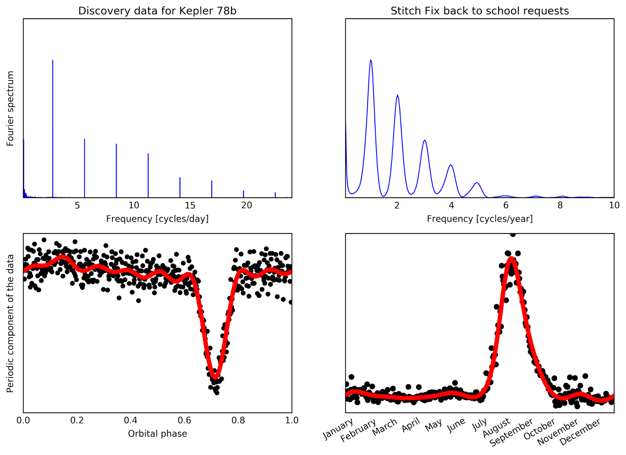
Comparison of the Fourier spectrum of the relevant data used to discover Kepler-78b (left) and the request notes that ask for “back to school” clothes (right). In blue on the upper figures, the value of the Fourier spectrum. On the lower part, black dots represent the aggregated data using the right principal frequency, binned down for easier inspection of the periodicity of the signal. In red, a super model that takes into account all the frequencies detected on the Fourier spectrum, which allow us to predict with high precision when new transits of the planets will happen and when we will get a higher demand of “back to school” clothes.
We can go one step further and fit a linear model that contains all of the different frequencies detected in the Fourier spectrum. This new model can be written as
\[S(t) = a_0 + \sum_{i = 1}^{N} a_i \sin{\left( \frac{2 \pi t}{P} i \right)} + b_i \cos{\left( \frac{2 \pi t}{P} i \right)}\]Where S(t) represents the periodic part of the signal (also known as seasonality) and N is the number of frequencies to use (4-6 will be enough). The same least square fit will suffice to generate the best fit model, the red line, that can be seen in the lower left corner of the figure. With such a model, we can calculate the time of transit with precision, and use that to plan future observations of this planet’s transits with other telescopes.
In the case of the fashion data, we can focus on a very common fashion trend, getting special “back to school” clothes. We can use data from the past few years to build the time-series described in the previous section. On the upper right part of the figure we can see the special Fourier spectrum built using GLM fits on that dataset, with a general structure that looks very similar to the Fourier spectrum of the exoplanet data. We can see that there is one main peak that corresponds to a one year cycle, as we could have expected since this fashion trend is seasonal and always appears before the end of the summer. The same pattern of peaks appears at multiples of one cycle per year, which means that the shape of the signal must be similarly non-sinusoidal. When we combine all the data used to build the Fourier spectrum (see lower left corner of the figure), we can see that the signal looks like the planet signal but inverted, and that there is a large demand for “back to school” clothes towards the end of summer.
The same super model can be built with all the detected frequencies, but this time using a GLM to fit the data, and we can see on the lower left corner of the figure that the model fits the data very well. This model can be used to predict that the peak demand every year will be during the second week of August, pretty much in line with the beginning of the school year.
Conclusions
As we have seen, things as different as exoplanetary systems and fashion have a pretty direct connection in terms of the statistical tools that we can use to study them. This connection is not unique, since some of the tools used in the frontier of fashion and Big Data come from other fields of Science and Engineering (see our data-driven approach to fashion design or how we optimize warehouse operations for example). Coming up with these parallelisms is one of the great challenges of Data Science, one that if tackled properly will certainly help to evolve the field at the same pace that it has been growing over the past decade.